Reductive groups: a rapid introduction

The goal of this post is to introduce, in a very informal way, the notion of a reductive group, and discuss some examples.

Preamble

Last term I gave a mini-course in a seminar here at Berkeley on the theory of linear algebraic groups with a focus on reductive groups. As part of that, I wrote up a significant set of notes (now in excess of 200 pages), which I have been wanting to finish and post. Of course, this is large undertaking, and so might take a while.

But, I just recently also gave a talk in a number theory seminar at Berkeley on essentially the same topic. The main difference was that this was a seminar on Shimura varieties (so mostly interested in the characteristic theory), and I only had an hour and a half (opposed to 6 hour and a half lectures). Consequently, many of the proofs, but more importantly beautiful details of the theory, were left off.

While this is certainly not ideal for someone wanting to get a very thorough, and deeply-rooted understanding of linear algebraic groups, I realized that it serves an equally important purpose. Sometimes one just wants to get an idea of what something is, to see what it’s used for, and what the main tools used in the subject look like.

Thus, for this reason, I’ve decided to essentially transcribe my notes into wordpress format, with some slight expansions. I do still hope, eventually, to post my long set of notes from the mini-course, but hopefully, as I mentioned above, this post will serve as a rough guide, or, at least, an amuse-bouche.

The main goal is just to understand the definition of a reductive group, and understand how one would show various basic examples of linear algebraic groups are, in fact, reductive.

Motivation

The topic of this post is reductive linear algebraic groups. Let us motivate our reason to care about such objects adjective chunk by adjective chunk.

Groups

There are many fancy reasons one can give as to why the groups in a given category are desirable objects of study. But, to be frank, they mostly boil down to one simple idea: groups are nice.

Namely, it’s a founding principle of geometry that objects enjoying a large sets of symmetries are generally much nicer behaved, and have a much richer theory, than those without such transformations. Groups then, in this light, are perhaps the most obvious source of objects with large sets of symmetries since any group acts simply transitively on itself by left translation.

Of course, really what we’re talking about are homogenous spaces, spaces with a transitive action by their automorphism group, or equivalently, quotients of groups. But, since groups themselves are the simplest type of such spaces, they are of initial interest.

Thus, an algebraic geometer should be interested in  algebraic groups for the simple reason that they provide, in some sense, the simplest type of geometric object. They are also the objects for which an abstract notion of symmetry can be studied algebraically. Less cryptically, if one has a flat projective -scheme , then it’s automorphism functor is representable, and thus a group scheme.

These are some of the reasons, amongst many others, that we care about groups.

Linear algebraic

But, the topic of this post is not about all algebraic groups but, instead, about linear algebraic groups. So, why do we make this restriction? There are two reasons that immediately come to mind.

First, linear algebraic groups are those that are accessible by representation theory. And since, after all, representation theory is one of the most powerful and comfortable tools available to mathematicians, this singles out linear algebraic groups as being a natural first subcategory of all groups to consider.

The second reason is that, for all intents and purposes, not much is lost by just studying algebraic groups. This is codified by the following famous result of Chevalley:

Theorem(Chevalley): Let be a perfect field, and a finite type group scheme. Then, there is a (essentially unique) decomposition:

in the category of group schemes, where is a linear algebraic group, and is an abelian variety.

Thus, in some sense, the entire theory of group schemes is partitioned into two subcases—the theory of linear algebraic groups, and the theory of abelian varieties.

Unfortunately, or very fortunately, these two subjects, while both extremely rich, are largely incommensurate. Namely, what essentially characterizes linear algebraic groups is that they have representation theory (in a sense made precise below) whereas every representation of a connected abelian variety is trivial.

But, even if one is entirely interested in the abelian variety side of this picture (which some number theory enthusiasts might believe) the study of such objects is greatly enhanced by the study of linear algebraic groups. One reason, to be remarked on in the next section, is via the theory of Shimura varieties (which, very roughly, are moduli spaces of abelian varieties).

Another, more direct reason, is via the theory of Néron models. Namely, an abelian variety need not admit an abelian scheme model . But, the very general theory of Néron models provides a smooth group scheme with generic fiber subject to some natural conditions.

Many of the properties of can be understood well in terms of the geometry and algebra of this group scheme and its special fiber . And, thanks to the theorem of Chevalley mentioned above, this is always broken into an abelian variety component and a linear algebraic group component. Thus, even if one wants to understand abelian varieties, one is often times forced to deal with linear algebraic groups.

As a concrete example of this, recall the following famous theorem of Néron-Ogg-Shafarevich (or, perhaps more appropriately, Ogg-Tate-Serre):

Theorem(Néron-Ogg-Shafarevich): Let be a DVR with perfect residue field, , and an abelian variety. Then, has good reduction (i.e. admits an abelian scheme model ) if and only if the usual Galois representation

is unramified for any invertible on .

This theorem is extremely important. Practically it comes up in many other parts of one’s study of abelian varieties over number fields (e.g. Shafarevich’s conjecture, the open image theorem, etc.). Philosophically, it says that the (étale) homology of an abelian variety is sufficiently rich enough to know the reduction type of —a very deep idea.

I bring this theorem up here since the proof of said theorem breaks roughly into two parts. First is an understanding of Néron models. The second is a general understanding of the structure of linear algebraic groups. Once one has those two things the proof is, in essence, ‘easy’.

Reductive

We come, finally, to the adjective ‘reductive’ a, at first, scary sounding concept.

Reductivity can be thought about in a very simple-minded way as the property of a linear algebraic group the guarantees that has ‘nice representation theory’. This is a bit of an oversimplification, but serves one well intuitively.

For the purposes of the study of Shimura varieties reductiveness has a much more concrete realization. Namely, once again only roughly, Shimura varieties can be thought about as moduli spaces of polarizable Hodge structures. Then reductive groups become an obvious part of the study since they are, in essence, the Mumford-Tate groups of polarizable Hodge structures.

If the second bit of motivation means nothing to you, and it might not, then latch onto the first since, historically, this was the motivation for the study of reductive groups. Especially since this niceness of representation theory makes reductive groups amenable to ‘classification’.

Basics

Basic results

Before we walk, we crawl. In our case here, that means that we should recall the very basic ideas and definitions in the theory of group schemes.

In particular, let’s start with the fundamental definition. Let us fix a field . We then say that a group scheme over consists of a scheme together with maps

and

and

such that the quadruple ‘is a group’. In fancier parlance, this means that group schemes are group objects in the category of schemes.

It is often times much more fruitful to think about group schemes through a functor of points lens. Namely, by Yoneda’s lemma, to give the structure of a group scheme (i.e. the maps , , and ) it is equivalent to give a functorial in group structure on for every -scheme .

In other words, for every scheme one has the contravariant Hom functor

and to give the structure of a group is to factorize through the forgetful functor . Thus, a group scheme over is a functor such that the composition of with the forgetful functor is representable.

Thus, in practice, and surely in this post, we will often times think about group schemes as just being group-valued contravariant functors on . We will, without comment, take for granted that these functors are, in fact, representable (when thought about set-valued functors) leaving the details of this to the reader.

Let us now give some examples of group schemes over :

• Fix a finite abelian group . Consider the functor which takes a -scheme to the group (where is the number of connected components of ). This is a group scheme over called the constant groups scheme with values in .
• Let be the group scheme over with functor of points given by . This is called the group scheme of -roots of unity.
• Let be the group scheme over with functor of points given by . This is called the general linear group. It is almost universally true that one denotes by and calls it the multiplicative group.
• Let be the group scheme which assigns to a -scheme the group . This is called the special linear group.
• Let denote the standard orthogonal pairing on for any ring . Then, we can consider the groups and which assign to a scheme those elements of which preserve this pairing in the case of , and those which preserve the pairing and have determinant in the case of . We call these the orthogonal group and special orthogonal group respectively.
• Now let denote the standard symplectic pairing on for any ring . We define two group schemes and which associates to a the subgroup of which preserves the symplectic pairing in the case of , and those which preserve the pairing up to a (fixed) unit scalar in the case of . We call these the symplectic group and symplecitic similitude group.
• We define the group scheme to associate to any the group .

Just as an example, in the above, is represented by and the general linear group by .

As one might expect, a morphism of group schemes is just a morphism which preserves the multiplication map or, equivalently, a natural transformation between their associated group functors.

So, let us now define our actual term of interest. We call a group scheme a linear algebraic group if is finite type and affine. The term is not a misnomer since:

Theorem 1: Let be a group scheme. Then, is a linear algebraic group if and only if there exists an embedding for some .

Here the embedding means a closed embedding of groups which is just a group map whose underlying map of schemes is a closed embedding.

Thus Theorem 1 tells us that linear algebraic groups are just closed subgroups of the general linear groups—they are groups with faithful representations. While the proof of Theorem 1 is not too difficult, there is something semi-subtle happening. Indeed, one can define a group scheme over any scheme , and the definition of a linear algebraic group still stands—finite type and affine. But, the analogy of Theorem 1 is open if one replaces by even something as simple as (although it’s known for DVRs).

Now, one could spend literally years trying to understand the geometry of a general group scheme, or even just of a linear algebraic group (cf. SGA 3), but that is not our goal here. Thus, let us suffice ourselves with two theorems concerning such geometry.

The first goes to show how the homogenous space property makes the study of groups much simpler:

Theorem 2: Let be a linear algebraic group. Then, is smooth if and only if is geometrically reduced. Thus, if is perfect, then is smooth if and only if it’s reduced. If has characteristic , then is automatically smooth.

One nice corollary of the above is the following. There are many theorems below which, personally, I find very exciting. They all say something of the form ‘the only class of groups which satisfy BLAH conditions are the obvious ones’. Now, usually this class BLAH of conditions is really natural except for the inclusion of ‘smooth’ which, often, seems like an afterthought. The above tells us that as long as we’re in characteristic we can completely ignore this condition—all groups are smooth!

Proof(Sketch): Obviously if is smooth it’s geometrically reduced. Conversely, if is geometrically reduced then is reduced. But, then it’s well known (cf. Tag 056V) that there is a dense open for which is regular. But, then for any other closed point one sees that is a smooth neighborhood of , and thus is regular. Thus, all the closed points of are regular, thus is regular, thus is smooth.

The second claim is a famous theorem of Chevalley.

To summarize this proof: smoothness happens on a dense open for reduced schemes, but groups are homogenous (every point has a neighborhood isomorphic to a neighborhood of every point) so this smoothness propagates over the whole scheme. This line of argument is very common.

The other geometric idea we’ll need is the notion of exact sequence, quotients, and the existence thereof. Now, this is one of the most complicated parts of the basic theory of group schemes—what does mean? This is, almost everywhere in scheme theory, a difficult question—quotients are hard.

In this context, we have the following definition though. Given a map of group schemes over the kernel is the naive kernel (i.e. it’s ) and is the fppf sheafification of the quotient presheaf .

The shocking, stupendous theorem is then the following:

Theorem 3: Let be a linear algebraic group over , and a closed subgroup. Then, exists. If is normal in then this quotient has the unique structure of a group scheme such that the canonical map is a group map.

This is surprisingly complicated result (see SGA 3), but one we’ll use freely through the rest of this post without much comment.

Let us explore the above point just a tiny bit since, frankly, it can be quite confusing. In particular, let us focus our attention on what might be the most confusing application of Theorem 3. Namely, let us consider two group schemes over (assumed to be characteristic for convenience). Namely:

where, of course, this quotient is taken in the sense of Theorem 3.

Now, let us begin by making the following surprising observation: . Namely, there is a canonical map and, in fact, it’s an isomorphism. Indeed, it’s a closed embedding of group schemes obviously, but it’s also a surjection since this can be checked on -points where its obvious.

While this is shocking, it’s made less so if we recall what really is. Namely, for a second, let us denote the group scheme as . Then, the first important thing to notice is that where, on the right, this is the ‘usual group’ . Why is this true? Well, it’s because  is the value on of the quotient presheaf of but is the quotient sheaf (in the fppf topology).

In fact, to cement this point, note that the association

is not even representable! In particular, it is not a sheaf, so that we really do have to sheafify (for which it’s then still not obvious its representable, which is the content of Theorem 3).

Indeed, let’s see why this is true when and . For notational convenience (i.e. not to confuse us) let’s denote the association by . Then, we’re trying to show that is not a sheaf for the fppf topology. If were an fppf sheaf, in particular an étale sheaf, then we’d have for any prime that

would be a bijection where acts in the usual way.

That said, note that

is in . Indeed, the non-trivial element of acts on this matrix by

but these two elements of are equal since . That said, this matrix is not in the image of . Thus, we see that is not a sheaf, and so, by fiat, not representable.

So, the question remains—what are the sections if not ? The answer, as one might guess, lies in étale cohomology. Namely, we have a short exact sequence of fppf sheaves

and thus for every we get an exact sequence

and thus an exacts sequence

for all .

Now, since we assumed that we’re working in characteristic  we have that

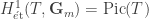
and from standard Kummer theory we know that we have a short exact sequence

Thus, we see that the natural map is an isomorphism whenever and . So, for example, we see that

for all .

It’s perhaps easier to understand the is using the fact that is isomorphic to the algebraic group which, for reasons similar to the above, we’ll denote (again, recall though, that we denote them differently here purely for cosmetic reasons). Namely, calling it is wise since (where this denominator is embedded as invertible scalar matrices). Let us denote this latter quantity by —again, it’s the quotient presheaf .

Again though, we have an exact sequence for all

But, now, we know that

and thus we see that

whenever .

Thus, as an example of this, we see that

even though is the group scheme !

Of course, we will stop denoting by and by —we’ll just denote them as and . That said, the above shows how subtle these notions are and how confusing the naming of them is. So, one should not sweat these details too much except to be very mindful that most group schemes like only necessarily give the correct group on geometric points (on other points one has to make a cohomology computation).

Applications to elliptic curves

To end this section, I’d like to give one way in which even these basic ideas allow us to better understand number theoretic questions.

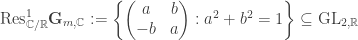
To begin with, let us say that a group scheme is a torus if (or equivalently ) is isomorphic to a power of the multiplicative group. Let us give some examples of these objects.

• Let denote the following subgroup of :

  

  Then, one can show that this is a -dimensional non-split (i.e. not just a power of the multiplicative group rationally) torus. It’s called the Deligne torus. One might recognize this construction since, in essence, this is just the standard embedding of into done on the level of schemes.

• Consider the following subgroup of

  

  then one can show fairly easily that this is a non-split -dimensional torus over . In fact, there is a pretty natural short exact sequence

  

So, how do tori help us understand number theory better? Well, the key is the following two theorems which, at first, seem intimidating but are really not:

Theorem 4: Let be a field. Then, there is a canonical bijection between the isomorphism classes of -dimensional tori over and the set where has the discrete topology.

Explicitly, this says that there is a bijection between -dimensional tori and the fields and the quadratic Galois extensions . What is this bijection? Well, goes to the split torus and goes to . Understanding this precisely won’t be important to our application at large.

But, one can make an even more powerful statement which, to me, is a truly spectacular, beautiful result that one would not expect should exist:

Theorem 5: Let be a perfect field and a -dimensional connected smooth linear algebraic group. Then, is one of the following:

1. .
2. 
3. for some Galois quadratic extension .

In particular, we deduce the following:

Corollary 6: Let be, as usual, a finite field. Then, up to isomorphism, there are only three -dimensional smooth connected linear algebraic groups over . They are , , and .

OK, this is nice, but so what? I’ve still not explained how this helps us understand something number theoretic!

So, finally, let us consider what is the beginning of many number theoretic jokes: so an elliptic curve over with bad reduction at walks into a bar…

But, really, let be an elliptic curve. Then, since has class number we can lift to a curve in a canonical way (its minimal Weierstrass model). We then define the reduction of at to be .

Now, it’s well known that , the smooth subset of , has the structure of a group (the same chord-tangent construction works). So, since is a smooth, connected, -dimensional group scheme over , and all curves are either affine or projective, we know that is either a smooth, connected, -dimensional linear algebraic group, or it’s still an elliptic curve.

Thus, by Corollary 6 there are four choices for what is. These four choices have names:

so the (at least to me) mysterious ‘four reduction types’ can be understood quite nicely in terms of the group schemes over a finite field.

Reductive group schemes

We now move onto the main course, the theory of reductive group schemes.

Before we begin in earnest, let us say, again, what the intuition is: reductive group schemes are those with nice representation theory. This manifests itself in characteristic zero in the following nice way:

Theorem 7: Let be characteristic . Then, a linear algebraic group is reductive if and only if is semisimple.

Here is the category of representations (i.e. homomorphisms into some general linear group). Thus, in words, the above says that reductive groups are precisely those groups for which every representation breaks up into irreducible parts. This is clearly a highly desirable property of a group and is the reason for the namesake ‘reductive’ (things reduce to irreducible pieces!).

Of course, in positive characteristic things get a little more sticky. There the notion of reductive and linearly reductive (i.e. all your representations are semisimple) diverge (the latter implies the former, but not conversely). But, for technical reasons, it’s the notion of reductiveness which stays more true to our ideals especially when concerned with classification theory.

For example since reductive groups are supposed to be ‘nice groups’ we’d hope that the most natural of all groups, the general linear group, is reductive. This is true, but in characteristic the group need not be linearly reductive. Thus, again for technical reasons, reductiveness and not linear reductiveness, is the correct notion even though, personally, I mostly think about reductive as meaning linearly reductive up to some fudge factor.

So, if linearly reductive is not the right notion we need to find some other way of defining reductiveness. The rough idea is to single out those groups with the worst representation theory, and define reductive groups as being those groups with no such part.

To this end, we make the following definition. A linear algebraic group is called unipotent if it satisfies any of the following equivalent conditions:

• It admits an embedding into

  

• All representations have a fixed point. In other words, has no non-trivial simple representation.

• It admits a decomposition

  

  with each normal in and is isomorphic to a subgroup of .

• If is also smooth, then there is the following equivalent condition. There exists an embedding such that (or, more properly, the image of this group) consists entirely of unipotent matrices (i.e. a matrix such that is nilpotent).

It should be noted that in this third criteria, if is smooth and connected (which is automatic if has characteristic ) one can take .

Let us give some simple examples:

• The group is obviously unipotent.
• The group is evidently unipotent by the third criteria.
• Assume that has characteristic . Let be the group scheme given by . One can think of as being the kernel of the Frobenius map given on points by . This is, of course, a group map because we’re in characteristic . Then, is unipotent since it’s a subgroup of .

We can see the second criteria as saying that has the worst possible representation theory. Namely, the only semisimple representation is the trivial representation! Thus, one might imagine that those which have good representation theory are those with no unipotent part.

To this end, let us define the unipotent radical of a linear algebraic group , denoted , to be the largest connected, smooth, normal, unipotent subgroups of .

The first non-obvious fact is the following:

Theorem 8: exists.

Let us give some examples of unipotent radicals:

• for any torus .
• .
• .
• .
• .
• Let denote the subgroup of of all upper triangular matrices. Then, .
• .

Let us also state one other basic property of the unipotent radical:

Theorem 9: For any separable extension one has that .

Thus, we might imagine that groups with nice representation theory are those with . So, to this end, we can now give a rigorous of a reductive group. Let be a linear algebraic group. Then, is reductive if .

Of course, the first thing that one might ask is whether we can remove this geometric condition—whether being reductive is equivalent to . If is perfect, so that , then this follows immediately from Theorem 9. If not, then this needn’t be the case. Lucky for you, dear reader, Brian Conrad et. al. has written an entire book about the topic called Pseudo-reductive Groups. Feel free to check it out! 🙂

So, we now have a bunch of examples of reductive groups:

• .
• .
• .
• .
• .
• .
• Tori.

and some good non-examples

• Any unipotent group.
• .

But, these claims are all rested upon the computations claimed above (and some that weren’t claimed), such as . Thus, we’d like to work towards understanding how such a computation can be made in the rest of this post.

But, before we move on to this, we’d like to discuss some basic properties of reductive groups and how one can understand them very well in the case when .

To begin, let us state the properties of reductive groups, in the abstract, we’d like to emphasize:

Theorem 10: Let be a linear algebraic group.

1. If has characteristic , then is reductive if and only if it’s linearly reductive.
2. is a torus if and only if is connected, smooth, reductive, and commutative.
3. The group is reductive. Thus, every linear algebraic group is the extension of a reductive group by a unipotent group.

We’ve already discussed 1. of the above theorem. Property 3. says that, up to the extension problem. all linear algebraic groups can be understood in terms of reductive and unipotent groups. Both type of groups are relatively simple—reductive groups have nice representation theory (and, in fact, a classification theorem!), and unipotent groups are just iterated extensions of .

We’d like to then just mention why 2. is true by discussing a more general fact:

Theorem 11: Let be a connected smooth commutative linear algebraic group. Then, where is unipotent and is a torus.

Thus, 2. of Theorem 10 follows quite easily. Indeed, in such a decomposition it’s evident that . Thus, (i.e. is reductive) if and only if , so that is a torus.

So, as stated above, let us finish this section with a look at what reductiveness looks like when .

The key definition is the following. Let be a linear algebraic group. Then, an involutive morphism is called a Cartan involution if

which is a Lie group, is compact. One can, in fact, show that, as the notion suggests, there is an algebraic group for which is just the -points.

The main theorem is then the following:

Theorem 12: Let be a linear algebraic group.

1. All Cartan involutions on are conjugate.
2. is reductive if and only if it has a Cartan involution.

Proof(Sketch): Let us say why one direction of 2. is true. Namely, suppose that has a Cartan involution. To show that is reductive it suffices, by Theorem 9, to show that is reductive. Since we’re in characteristic it suffices to show that is linearly reductive.

Let be any representation of . Let be a Cartan involution and let be the twist by . Note that we obtain a representation of the Lie group which, since it’s a compact Lie group, is semisimple. Since the -points are Zariski dense, one can use the decomposition of this Lie group representation to produce a decomposition of the -representation.

Let us give what is, essentially, the only example of a Cartan involution:

• Consider the involution of given by —inverse transpose. This is a Cartan involution since those such that are precisely the unitary matrices which, as is well-known, form a compact subgroup of .

Using the above ideas, we derive the following extremely pleasing result:

Theorem 13: Let be a linear algebraic group. Then, is reductive if and only if there exists a faithful representation whose image is stable under transpose.

Proof(Sketch): If such an embedding exists, then the restriction of to would give a Cartan involution of . The other direction is more complicated and requires some legwork of Satake.

This immediately proves that all the claimed examples of reductive groups above are reductive, at least in the case when . But, one can show that for a linear algebraic group reductiveness is equivalent to reductiveness of . Thus, we immediately conclude that all of the following groups are reductive over and thus reductive over any characteristic field: , , , , , , …

But, frankly, this feels like cheating. Namely, even though we have rigorously proven reductiveness we have done it by recourse to analytic techniques—the fact that all compact Lie groups are linearly reductive requires the existence of -invariant inner product, which, in turn, requires using the Haar measure (i.e. ‘average’ any inner product).

Thus, we’d still like to justify our calculations of as above using purely algebraic techniques, which is what we will aim to do.

Semisimple groups

Our goal of trying to understand computations such as so as to able to, in particular, give a characteristic independent way of proving is reductive, is going to naturally take us through the world of semisimple groups.

One can intuitively think about semisimple groups as being reductive groups with finite center or, equivalently, reductive groups which are almost adjoint (which, as in the theory of Lie groups, means that is injective). We will explain at the end of the post why ‘semisimple’ is not a misnomer since it won’t at all be clear from our initial presentation of such groups.

So, semisimple groups are going to come from forbidding large normal subgroups of a certain sort. But, instead of forbidding large normal unipotent subgroups we’re going to forbid large normal solvable subgroups.

So, we begin, as we should, with the definition of solvable. Namely, let be a smooth linear algebraic group. Then, we say that is solvable if either of the equivalent properties holds:

• The group is solvable.
• There is a filtration

  

  such that is normal in and is abelian.

One must be careful since these two are only equivalent when is smooth.

Let us give some good examples:

• Any unipotent group.
• The group —it has as as normal subgroup with quotient .

In fact, the second group above is fairly representative as the following shows:

Theorem 14 (Lie-Kolchin Theorem): Let be a smooth solvable connected group. Then, admits an embedding .

There are also some representative non-examples:

• .
• .

In fact, it’s not hard to show that

which certainly shows the result. Once one understands the slightly subtle notion of an algebro-geometric definition of commutator subgroup (which we discuss later in this post), the above can be made algebraic.

So, as stated above, semisimple groups are made by essentially restricting them from having large normal solvable subgroups. So, we need an analogue of which is supplied by the following. Let be a linear algebraic group. Define the radical of , denoted , to be the largest normal, smooth, connected, solvable subgroups of .

Again, the first non-obvious theorem is the following:

Theorem 15: Let be a linear algebraic group. Then:

1. exists.
2. for any separable extension

Let us consider some examples:

• , in other words its the scalar matrices.
• .
• .
• for any connected smooth solvable group.

Again, it’s not obvious how to actually make these computations—something we will remedy below.

So, with this setup we can easily make the definition of semisimple groups. Namely, a linear algebraic group is semisimple if . Similar comments concerning equivalence to hold as in the case of reductive groups. Namely, as long as is perfect this is equivalent to and in the non-perfect case one gets, what I assume, would be called pseudo-semisimple groups.

Some examples:

• .
• .
• which is defined as .

and some non-examples:

• Solvable groups.
• .
• 

Now, we want to develop some machinery that will allow us to actually make these computations. The first step in this chain is to discuss the notion of a Borel subgroup. Namely, a closed subgroup is Borel if it is connected, smooth, solvable and is maximal amongst subgroups of with this property.

The reason for needing maximality over is very much related to the following: Borel’s need not exist. Namely, a linear algebraic group which has a Borel is called quasi-split. It’s not hard to show that if then all groups are quasi-split but if is, say, then there are certainly non-quasi-split groups.

Checking that a group is Borel, and classifying all such Borels seems like a difficult problem. And, while it is, the following certainly makes it much more tenable:

Theorem 16: Let be a linear algebraic group.

1. All Borels are conjugate over .
2. A connected solvable smooth subgroup is Borel if and only if is projective (equivalently, proper).

Thus, for example, we can now give some good examples of Borels:

• The subgroup is Borel. Indeed, it’s evidently smooth, connected, and solvable. Thus, it remains to show that is projective. But, acts transitively on the complete flag variety with stabilizer of the standard flag being . Thus, . And, since is projective, it follows that is a Borel.

The reason that Borels are powerful in the computation of radicals and unipotent radicals is the following:

Theorem 17: Let be a linear algebraic group where . Then, the following equality holds:

Here the denotes connected component, and the subscript means take the reduced subscheme (which is still a group).

Proof(Sketch): Since is connected, solvable, and smooth it’s contained in a maximal such group which is necessarily Borel. But, since all Borels are conjugate, and is normal, is contained in every Borel so contained in their intersection. It’s then contained in the connected component since it’s connected, and contained in the reduced subscheme since it’s smooth.

Conversely, the intersection of all Borels is normal (since they’re all conjugate) and solvable (since this can be checked on -points). Thus, the intersection of the Borels connected component’s reduced structure is connected, normal, solvable, and smooth and thus, by definition, contained in .

We need one last tiny, obvious observation:

Theorem 18: Let be a linear algebraic group. Then:

Thus, we are finally prepared to justify some of the calculations we made above:

• We claim that and . It suffices to check this geometrically. To see this, begin by noting that, as proved above, is a Borel subgroup of . Thus, also, is , the group of lower triangular matrices. Thus, we see that which consists of diagonal matrices. Then, one can easily see that the only normal-in- subgroup of the diagonal matrices is which proves the claim.Note then that by Theorem 18 is . But, evidently, .
• We claim that . It suffices to check this geometrically, and to only check that . But, again, note that if we define and that . But, is just the diagonal matrices of determinant . The only normal-in- subgroup of this is just the diagonally embedded copy of . But, the largest connected reduced subgroup of is and since must be contained in this subgroup, the conclusion follows.

One can use similar ideas to do the rest of the computations that we claimed above. In particular, one can use this to prove the groups we claimed are reductive/semisimple really are so (independent of characteristic).

Let us end this section with some general calculation friendly results:

Theorem 19: Let be a connected reductive linear algebraic group over where is perfect. Then:

Here the subscript ‘‘ means the reduced subscheme which, because is perfect, inherits the structure of a group.

Proof(Sketch): We obviously have that , so it suffices to check the reverse inclusion.

Begin by noticing that is a torus since is reductive. Indeed, by Theorem 18 it’s clear that is reductive. But, then is a connected, reductive, solvable group which implies it’s a torus. Indeed, since is connected and solvable it has a subnormal filtration whose quotients are abelian, reductive, connected groups. But, by Theorem 11 this implies that has a subnormal filtration whose quotients are tori. One can show this implies that is a torus.

Now, the next key step is the following rigidity lemma:

Lemma 20: Let be a connected linear algebraic group and a torus. Then, any action of on is trivial.

From this, we conclude that the conjugation action of on the torus is trivial, and so is central. Thus, giving the reverse inclusion. .

With this, we can justify our intuition from the beginning of the section:

Theorem 21: Let be a connected linear algebraic group where is perfect. Then, is semisimple if and only if is reductive and is finite (as a -scheme).

Proof(Sketch): Suppose first that is semisimple. Then, since we deduce that . This evidently implies that is zero-dimensional, and so finite.

Conversely, suppose that is reductive with finite center. Then, being finite means that and so the conclusion follows from Theorem 19.

These theorems also allow us to try and understand semisimple and reductive groups in terms of their commutative subgroups. Namely:

Theorem 22: Let be a connected linear algebraic group and assume that is perfect. Then, is reductive if and only if the largest normal abelian subgroup is of multiplicative type. It’s semsimple if and only if its only normal abelian subgroups are finite étale.

Here, to be of multiplicative type means that, geometrically, one is isomorphic to product of tori and groups of the form for coprime to .

Proof: Suppose that is reductive and let be any normal commutative subgroup. Then, is normal connected and commutative, and so . As was shown in the proof of Theorem 19, we know that is a torus. Then, is a torus by fiat.

Now, as classically is known (see section 5.i of Milne’s notes on algebraic groups) there is a short exact sequence

where is a finite étale scheme (the group of components). Now, since is perfect this sequence splits (see 5.53 of loc. cit.) and since our groups are abelian we conclude that

But, is a finite abelian étale group scheme, and so multiplicative. The result follows.

Conversely, suppose that every normal abelian subgroup of is of multiplicative type. Then, in particular, is of multiplicative type and, since it’s connected, must be a torus. This then implies that

as desired.

Suppose now that is semisimple and let be any normal abelian subgroup. Then, is of multiplicative type (since is reductive). But, since we conclude that is finite, as desired.

Conversely, suppose that has only finite étale subgroups. Then, note that is reductive (by the previous case) and so by Theorem 19 . But, since is a normal commutative subgroup, this implies that is finite abelian étale. This implies that is trivial (this can be checked over where all finite abelian étale groups are constant).

This gives a fairly concrete way of discussing semisimplicity and reductivity of groups since, as is plain to see, it doesn’t require any of the more sophisticated notions of unipotent groups, solvable groups, etc. This is the perspective taken in notes such as this nice article..

The isogeny category

Alternative characterizations

In this section we’d like to discuss, without proof (or without the entire proof), some structure results about reductive and semisimple groups.

To begin we’d like to approach the question of finding ‘nice groups’ in a different way. Above, we essentially approached this question from the point of view that ‘nice groups’ meant groups with reasonably nice representation theory. But, there is another obvious perspective. Namely, in a subject like group theory we define an object to be ‘simple’ if it has no non-trivial subobjects, and this is one good definition of ‘nice’. Can something similar happen here? If so, how do reductive and semisimple groups fit into that picture?

Let us begin with some definitions. A group is called simple if it is non-abelian and has no non-trivial, proper, normal subgroups. The exclusion of abelian is largely because they ‘play differently’ than the other simple groups (in the same way that is the odd man out in the theory of finite simple groups).

Her are some examples:

• The group is simple for –this is not overly obvious. In characteristic it suffices to check that is simple in which case one can see this nice note of K. Conrad.
• The group is almost simple. Indeed, if is a non-trivial proper connected smooth subgroup, then the same would true of the image in which implies, by the previous bullet, that . Thus, every non-trivial proper normal subgroup of is finite (in fact, contained in !)
• The group is not simple.

Also, let us call a homomorphism of algebraic groups an isogeny if it is finite and surjective with kernel lying in . We say that two groups and are isogenous if there exists a third group and isogenies and .

Remark: What we have defined here is really called a central isogeny. The difference is moot if is smooth (e.g. if is characteristic ) but can differ in positive characteristic. This is not important for us here though.

Also, note that the inclusion of this in the above can be somewhat disturbing for those familiar with abelian varieties. Namely, if there is an isogeny of abelian varieties , then there is an isogeny of abelian varieties . Thus, the notion of ‘isogenous’ for abelian varieties is just the existence of an isogeny in one direction which, by the above statement, really is an equivalence relation. That said, while there is an isogeny there is no isogeny (because is simply connected and and thus the same definition as for abelian varieties wouldn’t work here.

Let us give an example

• The obvious projection map is surjective with kernel , and so an isogeny.
• The map sending, on -points, the pair to is an isogeny with kernel isomorphic to (specifically the kernel is pairs of the form where is an -root of unity). This example is indicative of the ‘general case’ of reductive groups.

Thus, with these definitions we can give the following pleasant rephrasing of reductiveness and semisimplicity in the isogeny category:

Theorem 23: Let be a linear algebraic group. Then:

1. is reductive if and only if is isogenous to a product of simple groups and tori.
2. is semisimple if and only if is isogenous to a product of simple groups.

This justifies the name ‘semisimple’ and also explains that, at least in the isogeny category, reductive and semisimple groups are precisely the ‘other type’ of ‘nice group’ one gets by decomposing groups into their ‘simplest pieces’.

We can’t hope to prove 2. in Theorem 23  here (it’s incredibly lengthy) but, if we assume it, we can give a fairly simple proof of 1.

To start, let us define a notion which is deceptively difficult. Namely, for a linear algebraic group we’d like to define the derived subgroup (also called the commutator subgroup) . Now, the naive guess is that we should define it as follows:

but this is wrong! For example, we would very much like that for any field we have the equality

Indeed, this is what happens on -points and so, of course, what should actually happen. But, for example one has that

This example, while silly, does highlight the fact that our definition of the derived subgroup needs to be slightly more thought out than just defining it ‘pointwise’.

So, with this in mind, we give the alternate definition. Namely, let us define the derived subgroup of a linear algebraic group to be the intersection of all normal algebraic subgroups of such that is abelian. Intersection here can seem a little dodgy at first glance, but it’s actually A-OK. Namely, take the scheme theoretic intersection of these in , and note that it’s still a subgroup scheme. Be careful though, don’t be fooled into thinking that we can just take the set-theoretic intersection of the and give it the smallest closed subscheme structure (i.e. the reduced structure). While this works swimmingly in characteristic noting that in the intersection of the smooth subgroups and which gives shows that things are slightly more complicated in positive characteristic.

One can put their minds at ease concerning this definition if is smooth and connected (which essentially all of our examples are). Specifically, one then has that is characterized as the unique smooth connected subgroup such that (and similarly with replaced by ).

Some examples of the above are as follows:

• .
• .
• for any abelian linear algebraic group .
• .
• .

And, as is plain to see, if is connected and smooth, then is solvable (in the sense used above) if and only if the derived chain

terminates in finite time. Indeed, since all groups in sight are smooth, it suffices to check this on -points. But, the fact that then completes the proof.

So, how does this help us with Theorem 23? Well, we have the following observation:

Theorem 24: Let be a connected smooth reductive group over , then is semisimple.

The key to proving Theorem 24 will be the following beautiful result:

Theorem 25: let be a connected smooth reductive group over where is perfect. Then, is finite, and .

Here means the smallest algebraic subgroup of containing and .

Proof(Sketch): To see that is finite, we may proceed as follows. It suffices to check finiteness over , so let’s assume that is algebraically closed. Note then that for any faithful representation we may, since is a torus, conjugate this embedding so that lands in the diagonal matrices of . In fact, we can decompose into to character spaces for the -action, say we decompose it as with acting by the character . In particular, for any we have that is of the form where is a scalar matrix (specifically with scalar ).

Note though that since we must have that lands in the centralizer of the matrices of the form with scalar, which is precisely the group embedded diagonally into . So, finally note that if then is both of the form and a commutator in which is equivalent to being in . But, the matrices are then both scalar and have determinant , which means that their entries are -roots of unity, of which there are only finitely many. Thus, is finite as desired.

To see the second claim consider the quotient this is possible since both and are normal (and thus so is the group generated by the two). Note that this group is semisimple since it’s a quotient of (which is semisimple) and also abelian (being a quotient of ). But, since it’s also connected, the claim follows from Theorem 19.

We can now prove Theorem 24:

Proof(Theorem 24, Sketch): Note that the map is finite surjective. But, is semisimple. So, suppose that is connected smooth and solvable. Then, evidently, its image in is connected normal smooth solvable and thus, since is semisimple must be trivial. This implies that and thus finite. But, since is smooth and connected this is a contradiction.

Thus, we can finally explain how 1. of Theorem 23 follows from 2. Indeed, consider the map

given, on -points, by . Note that this is, in fact, a group map since (again by Theorem 19) we know that . This map is surjective by Theorem 25 and has kernel which, again by Theorem 25, is finite and evidently central. Thus, is isogenous to . But, is semisimple (by theorem 24) and is a torus (by theorem 19). Thus, if we know 2. then certainly we can deduce 1.

For example, we already remarked that was isogenous to which is precisely the isogeny with . As we’ve already remarked is isogenous to the semisimple group  and is a torus, and thus a decomposition of (in the isogeny category) as a product of a simple group a torus is given by .

The isogeny theorem

Let us end this post with just a taste of the very in-depth classification theory that accompanies reductive and semisimple groups. This is, broadly, the theory of root data which is an entire subject onto itself. So, we’ll suffice it to state here one version of the isogeny theorem.

To state this correctly though, we need one more definition. Namely, we call a connected semisimple groups  simply connected if every isogeny , with connected, and whose kernel lies in is an isomorphism. In characteristic this second condition is automatic. Indeed, the action of on the finite kernel must be trivial since is connected and the kernel is finite étale.

The name can be justified as follows:

Theorem 26: let be a connected semisimple group. Then, is simply connected if and only if is simply connected.

Here denotes the analytification of —the associated complex Lie group.

Proof(Sketch): Suppose first that is simply connected. Note that any isogeny induces, in particular, a covering map . Thus, by assumption, this is an isomorphism, so is an isomorphism.

Conversely, suppose that is simply connected in the sense of semisimple groups. We aim to show that . But, since is Lie group we know that is a finitely generated abelian group and, consequently, it suffices to show that its profinite completion is zero. But, it’s profinite completion is, as is well-known, . Thus, it suffices to show that . But, if is a Galois étale cover, then it’s not hard to show that one can supply the structure of  a semisimple group such that this map is an isogeny, so it must be an isomorphism. Thus, as desired.

In fact, less obviously so (but in the same vein as the above theorem) is the following. Let be a perfect field and and let be a connected semisimple group. Then, there exists a a simply connected semisimple group and an isogeny called the universal cover of . It satisfies the property that for any other central isogeny , there is a unique factorization through . If one then defines , which can be shown to a finite connected commutative  group scheme, then one can show that if then is non-canonically isomorphic to (where, recally, one defines ).

So, with these definitions down, we can state one basic version of the isogeny theorem:

Theorem 27 (Isogeny theorem): Let be algebraically closed, and a simply connected semisimple group. Then, is isogenous to a product of groups where is an element of the following list:

1. 
2. .
3. .
4. One of several ‘exceptional’ groups.

One might then wonder how to parameterize the isomorphism classes of semisimple groups within a fixed isogeny class. The idea, roughly, is that there is a ‘largest’ and a ‘smallest’ member of each isogeny class, and so really one just needs to understand what’s in between these two members. Specifically, recall that if is any semisimple group then we have its universal cover which is, by fiat, the largest group in ‘s isogeny class. The smallest is taken up by the adjoint group of defined, as usual, to be . Moreover, the map is an isogeny, so we really only have to worry about finitely many such groups within a given isogeny class.

Note, moreover, that while the simply connected or adjoint groups in a given isogeny class are the obvious representatives, there really is no preferred representative between them. In particular, in Theorem 27 above list we gave the simply connected constituents of the isogeny classes of the groups involved. We could have also listed the adjoint constituents and said that was isogenous to a product of groups in the following list:

1. 
2. 
3. 
4. One of several ‘exceptional’ groups (which are now the adjoint exceptional groups).

which is really no different (and not wholly more enlightening).