A fun (enough) talk

This is a rough transcription of a talk I gave to a class of algebraic number theory students at UC Berkeley with the goal of trying to understand how one might bring to bear modern techniques in number theory/geometry on some classical questions. I have essentially kept the format the same, while adding a bit of extra material (and adding in their responses to questions I asked).

A warning

This talk was difficult to write for multiple reasons. Most relevant to the reader though was the unknown, and likely highly variable, backgrounds of the audience members. For this reason I chose to keep things as simple as possible and consequently, in the process, acquiesced quite a bit of rigor. I think that these mistakes are not so bad since it seems, to me, that any reader capable of identifying mistakes is likely able to see how to fix them. But, again, there are some informalities/inaccuraces.

What is the point?

So, everyone learning algebraic number theory for the first time is, ostensibly, interested in studying, well, number theory. An innocent enough statement, but it begs a much more complicated question: what is number theory? Namely, if a well-educated student of analysis (or even an algebraic geometer!) asked a number theorist what their subject was all about, what should the response be?

This is surprisingly non-obvious question. The answer largely lies in the way in which number theory distinguishes itself from many other subjects of mathematics. I think Hida has said it best (paraphrasing): number theory is a subject not determined by its methods, but by its desiderata—the problems it wants to solve. As an example, one can think of analysis as being the study of objects amenable to the method of limiting processes. Number theory has no such method from which its problems spring. Instead, conversely, its methods (as wide and diverse as they are) are determined instead by the type of problems that it wants to solve.

So, let us rephrase the question: what things does number theory seek to solve/understand?

Remark: At this point I opened up this question to the audience—legitimately interested in what they might say. Unfortunately, I didn’t really get any real response.

The fact that none of you responded is, in my opinion, somewhat typical. Number theory is plagued by a serious discrepancy between its historical perspectives and its modern ones. For example, here are some ‘classical’ answers to the above question:

• Number theory is the study of primes and their distribution.
• Number theory is the study of cryptographical systems.
• Number theory is the study of Diophantine equations.

All of these perspectives are emphasized, for example, in a first undergraduate course on number theory and are what the lay mathematical student (someone that is not interested particularly in number theory) might say.

That said, while these are the classical perspectives on the goals of the subject, things have changed. One more modern perspective on what the ‘goal’ of number theory might be is the following:

• Number theory is the study of the absolute Galois group as a (topological) group and the study of its representations.

For example, the all-consuming web of conjectures known as the Langlands program (what both me and your teacher, my adviser, study!) is concerned with relating the representations of to algebraic geometry and (harmonic) analysis.

Moreover, the methods and techniques of the course you are currently taking are focused (implicitly) on this more modern perspective. Indeed, the usual big reveal of a first course in algebraic number theory are the results umbrellaed under the name Class Field Theory which, in all actuality, are just a summary of the character theory of and (implicitly) relating such characters to objects of an algebro-geometric and (harmonic) analytic nature.

This all being said, it is somewhat perverse (as well as a bit jarring) to wholeheartedly embrace this modern perspective without understanding its connections to the more elementary, naive questions that gave birth to it. Less pompously, it’s a bit of a shock to see how different the seeming goals and methods of an undergraduate course in number theory differ from that in a graduate course (let alone the cutting-edge research in the field).

Thus, the goal of today is to try and give some indication as to how this modern perspective of algebraic geometry and the study of and its actions (representations are just linearized actions!) actually aid the study of the most fundamental of the above ‘classical’ subjects: Diophantine equations.

Why Diophantine equations?

Before we undertake our journey in earnest, let us begin by explaining briefly why Diophantine equations are of interest to a modern number theorist.

We begin, as we should, by recalling the definition of a Diophantine equation. Namely, a Diophantine equation is an equation of the form with and where we require that . In words, Diophantine equations are the study of the integer roots of integer polynomials. Of course, even though we’ve chosen to focus on a single equation, one should consider simultaneous integer solutions to a family of integral polynomials as Diophantine equations as well.

Let us now give some classic examples of Diophantine equations, in increasing level of difficulty, and roughly how these equations are tackled:

• Pell’s equations: where is some fixed square-free integer. Such equations are taken care of, quite neatly, by the study of continued fractions and the study of the units of the ring (which is the ring of integers of if ).
• Catalan’s equation: where are fixed. This has the only solution (incredible!). This was solved by Mihalescu in 2002 using an incredibly clever argument which does not use much more than the number theory learned in this course.
• Fermat’s equation: with fixed. The solutions for and are explicitly parameterizable (see below!), and for there are no non-trivial solutions (i.e. solutions where none of or is zero). This was finally proven in the mid ’90s thanks to a huge number of people, most notably being Wiles, Ribet, Frey-Hellegourach, and Mazur. The solution was a tour de force of modern arithmetic geometry, which relied most pivotally on proving a small case of the aforementioned Langlands program.

All of these are incredibly interesting—Catalan says that no two consecutive integers (save and ) are perfect powers, and Fermat’s equation says that (except for and ) the sum of two -powers cannot be an -power—but why are Diophantine equations interesting in general? Why are they worth trying to study systematically, and not focusing on particular equations of interest?

Well, to begin with let’s drop all pretense and give what might be the most obvious answer to ‘what is the point of number theory?’: it’s the study of the integers . But, the study of with what structure? Depending on what your goal is the answer might be as an ordered ring but, for most purposes, the real goal is just to study as a plain ring. How then do Diophantine equations help us in this goal? The (soft) answer lies in the classic theorem of Yoneda. Namely, recall that the Yoneda philosophy tells us that if we want to study as a ring, we should study the sets for all rings . Well, any ring looks like for some (possibly gigantic) set of variables and equations . The set is nothing more than the set of solutions to the diophantine equations . Thus, the study of Diophantine equations, if you buy into the Yoneda philosophy, is equivalent to the study of as a ring.

Remark: Of course, the above is patently imprecise. Namely, the key aspect of Yoneda’s lemma is that you don’t only know as sets for all but that you actually know the functor or, in other words, how the solutions to these Diophantine equations all relate. Of course, this talk was not meant to be that precise in the first place.

What would a systematic study look like?

Now that we have (hopefully) convinced ourselves that Diophantine equations are worth our study, we need to decide how to systematically study Diophantine equations. Indeed, what the last part of the previous section told us is that to really understand we can’t study specific Diophantine equations (like the three listed above), we study them ALL. But, as you’ll notice, all the specific Diophantine equations above had very specific means of attacking them. If we hope to say anything general we thus need to develop a systematic way of studying Diophantine equations. But, what would this look like?

Let us begin by introducing a little bit of notation. Namely, if and is any ring, let us denote by the following set:

This terminology seems, at the start, to be nothing more than a convenient tool to discuss polynomial solutions. That said, just like the innocuousness of the Lagrange symbol, this simplicity is deceptive as the shift of thinking of the polynomial solutions for one ring (e.g. ) to all rings is an epoch changing maneuver the surface of which we’ll only just scratch.

But, let’s back off from that highfalutin nonsense for a second. Namely, we said that we are interested in studying Diophantine equations and thus, really, we’re interested in studying sets of the form . The issue, of course, is that this is hard. The reason this is hard is that sets are so unstructured. A hallmark of mathematics is to exploit the extra structure of an object. Sets, unfortunately, do not have much structure. So, our first order of business will be to replace this highly unstructured set with an object for which we will have much more structure to twiddle around with.

To this end, let us begin by replacing with something slightly larger. Namely, we replace by . We do this mostly for matters of simplification (related to the fact that is a ‘simpler ring’ than ) but for the types of we care about we’ll see that the containment is essentially an equality. That said, while might be ostensibly nicer, it’s still just a set, and therefore we still need to make a leap to give us something more amenable to study.

To this end, we replace by an even larger set: the set . Now, again, this seems like we’re in the same sort of unstructured territory we’re so desperately trying to escape but, in fact, we’re not. Indeed, the set comes with something fairly sophisticated: a Galois action. Indeed, since has rational (integral) coefficients if then

is in for any . In this way we obtain a -action on . Moreover, the topological structure of is not ignored, in the sense that the action of on is continuous (when is given the discrete topology).  And while the passage from to might, in general, be ‘lossy’ (one can’t necessarily recover the former from the latter) the passage from to the continuous -set is not: (where the superscript denotes fixed points).

Remark: In a way that one can make pretty precise, the above step is like studying a topological space by studying the space (its universal cover) with its associated action. The claim about fixed points becomes the claim that a -equivariant map descends uniquely to a map .

Thus, we see that we’ve already passed from something incredibly unstructured (the set ) to something with an immense amount of structure (the continuous -set ). But, before we continue, let’s pause to consider what is, perhaps, the simplest example.

Namely, let’s suppose that , so that is a univariate polynomial. What then does the -set look like? Well, it’s clear that is a finite, discrete set with a -action. Moreover, we can describe precisely the orbit structure of this action. Namely, if factors over as with distinct irreducibles of degree , then will be and the orbits of the -action on will be precisely the sets as varies.

We can soup this picture up even more. Namely, the way that acts on this finite set gives a continuous homomorphism

which evidently factors through an embedded copy of corresponding to the orbit decomposition of the -set described above. We can soup this up even further. Namely, we can take the standard/tautological permutation

Less crpytically, letting have basis we get the representation by declaring that .

Remark: For those that know what this means, the above representation might have a more familiar form. Namely, consider as the scheme and choose an isomorphism . Then, under this isomorphism the above representation is nothing more than (the zeroth -adic cohomology of ).

This representation contains all the essential information about —its irreducible factors and so, in particular, its rational roots (what we’re really after!). But, moreover, the representation provides an incredible tool to study the extension . Indeed, it’s clear that actually factors over and, in fact, gives a faithful (injective) representation . One can then try to completely understand properties of the extension by studying this representation . For example, we can entirely characterize the set of split primes (which completely characterizes by Chebotarev density) as follows:

where, of course, the above only really makes sense for unramified .

This is great. Namely, it allows us to study the -set and the extension using the incredibly rich theory of representations of finite groups (namely representations of the group ). Thus, at least in this case, we’ve eschewed the bonds of unstructured sets and donned the incredibly powerful wears of finite group representation theory—quite the upgrade!

Unfortunately, the above doesn’t quite work for general (i.e. not univariate ). Namely, we can still pass from the set to the continuous -set , but the next step is bound for failure in general. Namely, we built this representation from the tautological representation of , and for more general this set is going to be (countably) infinite. And, as one knows, the study of infinite-dimensional representations isn’t very useful/tractable without more structure. We need to develop a more sophisticated technique if we hope to proceed further.

Remark: One of the students in the class asked “Why not try to study these infinite dimensional representations using techniques of functional analysis?” To this I responded as follows. This is not a terrible idea, but the naive approach is not going to work. Namely, if we want to study representations into things like Hilbert spaces, we generally need our group to be sufficiently ‘analytic’. So, for example, one can study such Hilbert space representations for things like Lie groups since, after all, both are objects of a complex analytic nature, and thus are likely to have something interesting to say to one another. Trying this for our group is bound to fail in a literal sense since is ‘anti-analytic’. That said, trying to study by studying Hilbert space (with a small caveat) representations of a related group is the entire premise of the Langlands program!

So, if we’re not going to be able to use the naive definition of representations for general , then how shall we proceed? We begin by making an observation about one of the benefits that having very complicated gives us. As an example, let’s consider the polynomial . Then, as said above, is infinite. But, something spectacular happens here. Namely, if we enlarge even further something magical appears. Namely, if we replace with a clear-cut advantage of this case over the univariate case occurs. Namely, in the univariate case the -points are still just a discrete set of points. But, in the case of our current we get that is —the twice punctured plane. A gloriously rich topological object.

To this end, for any , let us give the structure of a topological space by considering it as a subspace of with the obvious embedding . Then, we see that what non-univariate polynomials lack in the naive amenability to representation theory, they make up for in having rich, intrinsic geometric structure.

With all of this structure uncovered, we can say (very broadly) how the systematic study of Diophantine equations goes. Namely, given we study through the continuous -set , the geometry of , and their interaction. This then creates a subject where one studies Diophantine equations by a mix of number theory and algebraic geometry which, in modern parlance, would be called arithmetic geometry.

We will come back to how this all relates to studying and its representations. But, before we do, we’d like to give a concrete example of using a mix of geometry and number theory to study a particular family of Diophantine equations.

An extended example

The example

So, as we said at the end of last section, we seek now to exploit our newfound methodology to study Diophantine equations to at least indicate how a natural class of such equations can be studied. What class of equations? Well, let us remark that in basic number theory the amount of honest Diophantine equations one solves is remarkably slim. To wit, this past summer I taught an elementary number theory course at UC Berkeley, and the only class of Diophantine equations I was able to solve was linear Diophantine equations in any number of variables. This is exceedingly simple, and essentially comes down to the Euclidean algorithm. The rest of the term was then, in fact, not studying Diophantine equations but ‘models’ for Diophantine equations: equations over finite fields.

Thus, any non-linear family of Diophantine equations is of current interest to us. So, with that being said, our goal is to use our broad methodology to prove the following:

Theorem(Legendre): Let be non-zero and pairwise coprime. Let be defined by . Then, the Diophantine equation

has a non-zero solution if and only if:

1. Not all of and are the same sign.
2. The number is a square modulo , the number is a square modulo , and the number is a square modulo .

Moreover, given one non-zero solution there is a natural way to parameterize all the solutions.

Note that this theorem is actually incredibly useful, because the theory of Quadratic Reciprocity gives us an incredibly powerful, quick means of checking 2. above.

So, before we dive into how geometry and number theory unite to prove Legendre’s Theorem, let us remark why this is, in some sense, the ‘next simplest example’ of equations after the univariate case. Of course, this may seem strange—how is this the next obvious case after the univariate case?—but as we’ll see, our lens by which to view Diophantine equations makes this precise.

So, towards this end, let us note that the set has a lot of redundancy. Namely, given any and any one obtains another solution just by the virtue of the fact that is homogenous. Note that this ‘line’ of solutions really shouldn’t be thought of as different solutions and the more fundamental object should be something like . So, to this end, if is a homogenous polynomial then we define . Note then that one immediately has .

Remark: For those that know what this means, note that this is technically the wrong definition of for general . Namely, we’d like to imagine that is just the projective scheme but the -points of this are not, in general, just . The issue is that this projective scheme is essentially the  moduli space for the quotient and, of course, in general we don’t expect quotient sheaves to have -points the quotient of the individual -points. The issue, as one can quickly deduce, lies in . But, this is not really going to be of interest to us since we’ll be dealing primarily with local rings .

Note that, just as in the case of one has that has a continuous -action and is a topological space (namely one takes the quotient space ).

So, with this in mind, we can explain why the polynomials are the next obvious choices after univariate polynomials. Namely, note that if is univariate then is a discrete topological space or, equivalently, a -dimensional compact complex manifold. There is an obvious parameter to tick up here: the dimension. So, the next obvious polynomials to look at are those such that is a -dimensional compact complex manifold. But, even amongst -dimensional compact complex manifolds there is a simplest. Namely, by the classification of compact orientable surfaces (of which every complex manifold is) there is a parameter given by the number of holes, the genus . The simplest one is then the surface of genus : the Riemann sphere .

Now, it seems obvious that the next obvious class of polynomials we should study are those such that is the Riemann sphere. Unfortunately, no such exist. That said, there are homogenous polynomials such that is . In fact, one can show that is means that (up to isomorphism) our polynomial is one of the as in the preamble to Legendre’s theorem. Thus, Legendre’s theorem really is the next logical step in our study of Diophantine equations.

Remark: Two remarks are in order for those that know what this means. First, the above statement really concerns not as a finite-type -scheme but its generic fiber over . Moreover, to make the above claim correct, we can’t have that is just topologically the Riemann surface, we also need that it’s the Riemann surface as a complex analytic space: that is . If we assume that is smooth then homeomorphism is enough, but the cuspidal cubic is not one of the and has analytification homeomorphic to .

The proof of the above claim is pretty simple. Namely, any such must have that (defined as its associated projective scheme over ) it a smooth geometrically integral genus curve. One can then show that for any such curve one obtains an embedding by considering (the inverse of the canonical bundle) which follows easily from Riemann-Roch. One then realizes is a hypersuface in which, by genus considerations, must be degree . The explicit form then follows from the elementary diagonalization of quadratic forms.

The fact that can never be follows from the standard fact about analytifications: that the analytification is compact if and only if the scheme is proper. By design is affine, so if it is also proper, then it’s finite. But, then is a finite set of points.

The geometric part

So, now that we see why the Diophantine equations addressed by Legendre’s theorem are the next logical step after univariate polynomials, we can begin to try to understand how one might prove the theorem itself. Let us first address the geometric side of the picture—the claim that one can use a single non-trivial solution  allows one to parameterize all the solutions of the Diophantine equation. Indeed, to show this we will exploit the geometry of at least morally—we’ll be exploiting the geometry of the scheme which is, essentially, the same thing.

So, to make this claim precise, let us assume is one of the equations from Legendre’s theorem and that is given. We then define a bijection

as follows. We can imagine as being a subset of . In particular, it looks like a subset cut out by a degree equation. For any point there is a unique line in passing through and . Map to the point in which is the slope of the line . Of course, we think of as having slope and so maps to . One can easily check that this map is surjective, and a basic verison of Bezout’s Theorem (which can be proven topologically/geometrically) says that if then —indeed, if then would intersect at at least three places (namely ) and this is impossible since the total number of intersection points of a subset cut out by a degree equation and a line is . This gives the desired bijection.

Remark: This is much nicer if one can draw a picture illustrating this point.

For those that know what this means, this is just the isomorphism given by the line bundle .

As an example of this, one can check that for and point one gets that the bijection from above shows that the rational points of (besides ) are essentially of the form 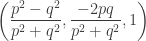where denotes the slope in reduced form. The integer solution in in the class of this point is . This should look familiar and, indeed, is just the set of Pythagorean triples, and this geometric procedure produces the usual parameterization of such triples.

The arithmetic part

Now that we have taken care of the geometric part of Legendre’s theorem, we need to explain the arithmetic part, the condition for which has a non-zero solution or, equivalently, for .

The motivation

The beginning is, in fact, also geometrically minded. For the next two minutes I will assume that people in the audience have basic familiarity with algebraic geometry. For those that do not, don’t fret, the conclusion will not have a lick of algebraic geometry in it—we’re just talking motivation.

So, it’s clear that from (thought about as the projective scheme ) we get a map . We can then think of as sections of this map . Now, if one is trying to build a section of a map of topological space, a common technique might be to try and build, for each , a section of where is a ‘very small’ neighborhood around . One then tries to glue these sections together to get a global section . So, if we try to analogize this property for we want to, for each prime , build a section from a ‘very small’ neighborhood of in .

The question then comes what a ‘very small’ neighborhoood of in might look like. The Zariski neighborhoods are too coarse, and so one needs to opt for something else. Namely, we think of a sufficiently small neighborhood of a point as being a neighborhood so small that properties of something at should extend to properties of that entire neighborhood. In other words, we want a neighborhood of such that the only obstruction to something in that neighborhood is an obstruction at . Since we’re thinking about polynomial equations, we think of an obstruction as being the lack of a solution to a polynomial equation . So, what does it mean for an equation to be unobstructed ‘at ‘?

Well, the naive guess is that it means the polynomial doesn’t have a solution modulo . But, this isn’t good enough. Namely, the prime gives more chance for obstruction than just modulo . What about modulo ? What about modulo ? It then seems reasonable to guess that unobstructed ‘at ‘ means that the polynomial has a solution modulo for all .

So, this ‘very small’ neighborhood should have the property that being unobstructed at is the same thing as being unobstructed in this neighborhood. Since we’re dealing with algebraic geometry, the neighborhood should be the spectrum of some ring , and reinterpreting this last sentence means that a polynomial equation should have a solution in if and only if it has a solution in for all . This is exactly describing the ring of -adic integers.

So, a ‘very small’ neighborhood of in is . Thus, a section of ‘very close’ to should mean a section of or, in other words, an element of .

Thus, the rephrasing of the geometric question of whether we can glue local sections to global sections is whether or not we can glue the elements of together for all to obtain a point of . In fact, one should also include in this setup. Indeed, given the function field of a curve , the points of correspond to the valuations on and the valuations of are , which corresponds to , for all and which corresponds to .

So, concretely, the question becomes whether or not for all valuations (define ) implies that is non-empty. If satisfies this for a homogenous we say that satisfies the local-to-global principle (or Hasse principle). Of course, there is no reason, a priori, to even expect this. Indeed, even for the sections of a map, one at least expect to impose some compatibility conditions on the overlaps of these local sections and the local-to-global principle doesn’t require the analogue of such compatibilities (what would that even mean?).

That said, let us see that the claim that the polynomials satisfy the local-to-global principle completely solves the first part (the criterion for non-zero solutions) of Legendre’s theorem. Indeed, we claim that the conditions stated are precisely the same as requiring for all . For example, 1. is easily seen to be equivalent to the claim that .

Suppose now that is a prime that does not divide any of or . We then claim that in this case without any effort whatsoever. Indeed, note that and the multi-variable version of Hensel’s lemma (that does exist!) tells us that the reduction map is a surjection. Thus, it suffices to show that . There are several ways to do this, but one very clear one is the following. Since are non-zero modulo we may assume (by dividing through) that . We are then trying to find the number of non-zero solutions to in and, in particular, show it’s non-zero. But, it suffices to show that there’s a solution to . But, this is equivalent to showing that the elements of of the form and the elements of the form have to have an element in common. But, note that since are non-zero each has precisely elements expressible in that form, and so if they had none in common, there’d be elements of , which is ridiculous. Thus, has a non-zero solution in and thus as desired.

Finally, let be a prime that divides one of . Note that by our assumption on the greatest common divisors of the (which is really no condition by dividing out any common divisors—if two of the coefficients is divisible by , so must be the third) we know that will divide precisely one of the . Let’s assume, without loss of generality that . Now, note that we want to begin the argument as in the previous case by using Hensel’s lemma. But, unfortunately, is not smooth over . So, to make things work, we instead work with defined as the those tuples in with non-vanishing -coordinate (or, in algebraic geometry language, where the intersection is happening in ). Note then that is, in fact, smooth over (over the non-smooth points of occur on the complement of !). Thus, by Hensel’s lemma it suffices to show that is non-empty. To see this we need to show that there is a solution to with . But, note that this is possible since is a square modulo so that and thus, by the multiplicativity of the Legendre symbol, is solvable. So, if is such a solution then evidently , , and work. Thus, is non-empty as desired.

The local-to-global principle

So, now that we’ve reduced Legendre’s theorem to the local-to-global principle for polynomials like we finish by applying some interesting number theoretic results to deduce the desired property. Namely, we will introduce an interesting object that will come later on in this course, and explain how its properties (that you’ll discuss) actually prove the local-to-global principle for the polynomials .

So, to this end, we take an ostensibly ninety-degree turn. Namely, for any field let us define a central simple algebra over to be a (possibly non-commutative) -algebra with the property that is isomorphic to as an -algebra for some . Let us say that two central simple algebras and are equivalent (written ) if there exists integers and Such that as -algebras. Finally, let the Brauer group of , denoted , the group of central simple algebras over up to equivalence, with group operation being tensor product. The identity of is the equivalence class of . Finally, we say that a central simple algebra is split if it’s equivalent to .

Remark: If you know what this means, .

Now that if one has a map of fields one obtains a map of Brauer groups given by . Indeed, it’s fairly easy to see that is a central simple -algebra since

and one can check that this map is, in fact, well-defined (i.e. if then ).

Our goal in this section is to explain how to use the Brauer groups, and their properties for local/global fields, to prove the local-to-global principle for the ‘s. This is, in some sense, a gross over-complication of the matter. But, our reasons for doing this are three-fold:

1. The whole goal of this post was to explain how ‘serious’ modern number theory that will show up in this course can be used to answer concrete questions—the below is a perfect example of this.
2. The proof of the below (while dramatic overkill) gives a much more conceptual understanding of why the local-to-global principle holds for the . There is a way to prove the local-to-global principle for ‘s using ‘elementary techniques’ (see here for instance), but they don’t really explain how the result fits into the larger context of abelian reciprocity laws/class field theory.Specifically, they don’t really explain in any essentially complete way why these Diophantine equations (and not many others) satisfy local-to-global principle. The stated result below should be thought of as the ‘true’ local-to-global statement, and the local-to-global property for our ‘s comes from a coincidental (or deep?) connection to central simple algebras.
3. The below method actually is (essentially) equivalent to a local-to-global result for Diophantine equations of a much more general form. Namely, let be homogenous polynomials in the same number of variables, and consider the Diophantine equation —the simultaneous Diophantine equations (for people that know what this means one should take ). Let us call this set of Diophantine equations Brauer-Severi if there is a (complex analytic) isomorphism (where ) which restricts an isomorphism (for those that know what this means, we just mean that ). Then, the below results can be (mostly) summarized as the claim that Brauer-Severi Diophantine equations satisfy the local-to-global principle. This is the correct light in which to view the result for the ‘s and really explains why their geometry is pivotal.

Before we go any further it’s worth discussing an explicit example of such objects. Namely, the Hamiltonian Quaternions are an example of a central simple algebra over . Indeed, one can check that . In fact, one can show that, up to equivalence, the only central simple algebras over are and so that .

So, why does this have anything to do with local-to-global principle for the ‘s? To begin, let us note that if we’re willing to take we can basically only consider the polynomial equations . Note then that with and . So, it suffices to explain how the polynomials relate to the Brauer group. So, to this end, let us define another concrete example of a central simple algebra over which, in a clear way, is a variation on a theme of the Hamiltonian Quaternions. Namely, for let be the following central simple algebra over :

with , , , and .

The theorem that then relates everything is the following:

Theorem: Let . Then, for any field the central simple algebra is split if and only if .

Proof(sketch): We first claim that is non-split if and only if it’s a division algebra. This follows at once from the well-known Artin-Wedderburn theorem. Indeed, since is simple with center we know that, as a -algebra, it’s isomorphic to with is a central division algebra. But, by dimension considerations we see that either is either or .

So, whether or not is split is equivalent to knowing whether it’s a division algebra. But, note that there is a norm map given by

One can check that where if . Thus, is multiplicative, and it’s pretty easy to check that if and only if .

Thus, the splitness of is equivalent to the existence of a non-zero non-unit of which is, by the previous paragraph, equivalent to the existence of (not all zero) such that . This looks like moderately close to the existence of a point in and, as it turns out (with a bit of algebra grease), that it’s true. You can look in the wonderful text Central Simple Algebras and Galois Cohomology (chapter 1) by Szamuely for the details.

Remark: The more conceptual reason for the above can be explained as follows. By a previous remark one can identify with . The short exact sequence of -groups

gives, by the connecting homomorphism and Hilbert Theorem 90, an injection of the form . But, note that and thus, by the theory of twists, classifies varieties over which become isomorphic to over —the Brauer-Severi varieties.

In particular, such a variety gives a class and thus, by the above, a class . Moreover, one can show that (i.e. isomorphic over not ) if and only if . Thus, we see that if and only if is trivial.

One can check, as was already done in the section labeled ‘The geometric part’, that becomes isomorphic to over and thus, putting this all together, we see that for every and any field one can associate some class in such that if and only if is split (i.e. trivial). As one might guess, is the central simple algebra with and .

So, from this we see that the local-to-global principle becomes equivalent to the claim that is split if and only if is split for all valuations of . So, how does one go about doing this?

The key is the following result that will be proven in this class:

Theorem(Fundamental sequence): There are isomorphisms and such that the following sequence is exact:

where and is .

This is an incredibly deep theorem. It contains within in it quite a bit of the wreckingball that is Class Field Theory. As an example, the fact that is trivial contains within it all the reciprocity laws (quadratic, cubic, Eisenstein) from elementary algebraic number theory. The proof comes from a detailed proof of the cohomology of the ideles of finite extensions of .

In particular, we see that this deep number theoretic result contains within it also the local-to-global principle for the polynomials . Indeed, taking and we have already observed that the local-to-global principle for is equivalent to the fact that is split if and only if is split for all . Using the terminology from the above theorem this is equivalent to the fact that is split if and only if is split. But, by the definition of the Brauer group this follows from the injectivity of .

In fact, we actually get something stronger from the above theorem. Namely, one can quite easily show that for each that the element is -torsion (prove this for yourself!). So, in particular, what we see is that if is non-zero, then it must be tuple of the form with each equal to (in which case it’s split) or (in which case it’s not). But, noting that we actually conclude that the number of places with is actually even! In particular, if we know that is split over , in other other words , for all but one then, in fact, is split over every and thus, in particular, . So, we have actually proven something stronger than Legendre’s therem.

Conclusion

We see that Legendre’s theorem, perhaps the most basic of all non-trivial Diophantine equations, requires (in its ‘correct’ proof) a true modern perspective: the combination of number theory and algebraic geometry—it requires arithmetic geometry. Quite amazing!

What comes next?

So, now that we’ve handled the Diophantine equations as in Legendre’s theorem, what type of equations come next? Using our previous discussion as a clue, we might try to look for polynomials such that are the next most complicated -dimensional compact complex manifolds: compact Riemann surfaces of genus .

These are, essentially, the so-called elliptic curves over . The study of their rational points, the solutions of the Diophantine equation, is a widely studied topic which comprises quite a sizable portion of modern research. For example, one can show that if is such an elliptic curve that is a finitely generated abelian group. We can then write where is a finite abelian group. Deep work of Mazur has identified the possible choices for : for and for . What the possibilites of can be is an incredibly intense area of modern research. It’s even hotly debated whether or not the possible are finite. Recent work of Manjul Bhargava shows that, probabilistically, half of the time and half of the time (this was one of the main reasons he received the Fields Medal). Moreover, there are deep conjectures (most notably the Birch and Swinnerton-Dyer conjecture) that relates this to important analytic objects (their -functions) which, due to Wiles, is the same thing as analytic objects coming from Harmonic analysis (automorphic -functions).

The next step might be to study with a curve of genus . The general theory of such is fairly sparse. But, thanks to Gerd Faltings we know an incredibly powerful qualitative result about the solutions to such Diophantine equations. Namely, Faltings shows that is always finite. An incredibly stunning results considering the incredible variety of examples it encompasses.

Remark: Not that most of this note has been rigorous, but it should be noted that the above paragraph was a discussion mostly in analogies. There are no with having genus for example—genus curves are not hypersurfaces. One should, if you know what this means, replace by  a smooth geomerically integral proper curve of genus in the above paragraph.

It should also be noted that we are largely, in the above, replacing the finite-type -scheme with its generic fiber.

After one is done with curves, the next step is to move onto Diophantine equations whose -points are higher-dimensional compact complex manifolds. Specifically, next up would be the study of proper surfaces (those Diophantine equations with associated complex points a -dimensional compact complex manifold). These are broken down into cases, similar to the partition of curves into their genus classes, by their minimal models. Namely, there is a classification of minimal surfaces (over , and this allows one to study the rational points of surfaces over by what their associated minimal surface over is. See this nice reference for a leisurely discussion of the topic.

Moving on from this point things get even more hard. Namely, for dimensions larger than there is no real geometric classification of the objects involved and so study by breaking them into similar classes seems impossible. Thus, there is currently no real general theory for Diophantine equations whose -points are compact complex manifolds of dimension greater than , only theory for such Diophantine equations of certain special forms (e.g. abelian varieties).

Relation to the ‘modern perspective’

I can’t resist, as a final note, explaining how this perspective on Diophantine equations allows us to more directly unite Diophantine equations with the modern perspective that number theory is the study of the group and its representations.

Namely, we saw that in the case of univariate polynomials that one could very easily associate a representation of that, in some sense, ‘tells all’. One of the reasons we then sought the refuge of the geometry underpinning ‘higher-dimensional Diophantine equations’ was that such a technique no longer proved to be possible. One may then wonder if one can actually exploit this geometry to remedy this situation—if we can use the geometry somehow to associate to Diophantine equations (of arbitrary dimensions) representations of which, like in the univarate case, give us insights into the solutions to the Diophantine equations.

So, the main impediment to extending what happened in the univariate case to higher dimensions was the lack of a natural finite-dimensional vector space attached to the Diophantine equation for to act on. Namely, we ostensibly made , for univariate, by creating a vector space in the dumbest possible way: using the tautological representation of . How might we analogize this to higher dimensions?

The key observation is that, in fact, one can think of the vector space showing up in the representation as actually coming from the geometry of . Namely, we saw that is nothing more than a set of discrete points with a continuous action of . Moreover, we can see that the representation essentially came from how permuted the connected components of this discrete space and, in particular, just acted on the free vector space on the connected components. In general, given a complex manifold , there is a name for the free vector spaces on the set of connected components of : the zeroth singular cohomology . Indeed, one can note that since is discrete that acts continuously on and thus, by the functoriality of singular cohomology, gives an induced linear action on . One can check that, as you’d hope, the -representations and are isomorphic.

This gives us a clear-cut way to try and attack the goal of associating to higher-dimensional Diophantine equations representations of . For example, if is a homogenous polynomial, then will be (in good situations) a compact complex manifold and thus, in particular, a well-behaved topological space. This allows us to associate to various complex vector spaces: the singular cohomology groups for . Of course, to make this be totally complete we will still need to define an action of on this space. Therein lies the rub. Namely, we have two difficulties that make this a much harder problem than in the discrete case. The first is that it is no longer true that (take for example). So, what we get is not an action of on but an action of . Of course, this action factors through on the subset .

The second, and more serious issue, is that we want to consider these cohomology groups of where we give the complex topology, NOT the discrete one. That said, only acts continuously on with the discrete topology, and acts wildly discontinuously on with the complex topology. In particular, since cohomology is only functorial for continuous maps, we seem completely doomed in utilizing the geometry to copy what happened in the univariate case for higher-dimensional examples.

In comes Grothendieck. It was Grothendieck’s brilliant genius to realize that one can fix the above, by understanding that the singular cohomology of can, in some sense, be obtained by algebraic methods and, in particular, in a way that allows one to actually have act on this singular cohomology. This is the modern masterpiece that is the theory of etale cohomology.

Let me briefly explain what this looks like. Grothendieck realize that to any scheme (thought of as a ‘geometric space associated to a set of equations’—think or ) one can associate certain vector spacess, denoted . Moreover, what Grothendieck shows, and this is the pivotal part, is that these cohomology groups are functorial in the scheme. In particular, if is a scheme obtained from a Diophantine equation then one has an operation, known as base change, which gives a scheme (this is much like ) and this has an action of (much in the same way that had an action of ) and thus, by Grothendieck’s wonderful machine, we obtain an action of on which is, in fact, continuous if one gives the cohomology group the natural topology of an vector space.

What does this have anything to do with the geometry of ? Well, Grothendieck and Artin showed that one has a natural isomorphism which, since , implies that (at least after choosing an isomorphism ) that . Thus, by Grothendieck’s wonderful machinery, and the beautiful result of Artin, one can define an action of on , but even better, a continuous action of on .

Thus, utilizing the geometry of the Diophantine equation and its arithmetic properties (i.e. viewing it through the lens of arithmetic geometry) one can associate to it a (continuous) representation of and, as promised, this enhances the study of the Diophantine equation. To elaborate on this would take many, many hours but suffice it to say that the representation contains within it much of the information of the Diophantine equation (e.g. the number of solutions of the equation modulo ). As an example, the fact that is a direct consequence (with the general theory at hand) of the fact that .

Moral of the story: learn schemes

So, let’s summarize all of what happened above. If one wants to study a Diophantine equation, there are many methods of attack for specific types of equations, but no general approach. This is undesirable. In particular, one would like to develop a method to study such Diophantine equations in a systematic way that ties into the modern number theoretic goal of studying and its representations.

One achieves this systematic approach by trading an unstructured set of solutions (e.g. or ) for a -set and a geometric object (e.g. and ) and studying the Diophantine equation between the study of these two separately (number theory and algebraic geometry) and their interaction (arithmetic geometry).

We saw a key example of this in trying to understand quadratic Diophantine equations. We were able to, in Legendre’s theorem, give a fairly satisfactory description of their structure. But, to do so, required that we view such Diophantine equations both as a geometric object (namely ) and an object of number theory (a class in the Brauer group ). Only by combining these approaches were we truly able to give our desired description.

Moreover, in the end, we indicated how this general arithemetico-geometric approach to Diophantine equations ties into the other modern perspective on number theory (the study of continuous representations of ) by explaining how the geometry allows us, thanks to the great work of Grothendieck (and many others, including Artin), associate to any Diophantine equation such a representation which, as hinted at, contains an immense amount of information about the Diophantine equation. Thus, the modern study of number theory (the study of Galois representations) does insert directly into the classical desire to study Diophantine equations.

Finally, it’s worth mentioning that all of the above is very neatly organized in modern algebraic geometry. Namely, it was the vision of Grothendieck and his collaborators to be able to neatly package the idea that from equations one can obtain a geometric and arithmetic object. Namely, they defined the notion of schemes which, in essence, captures both the arithmetic properties of the -set and the geometric properties of the topological (complex analytic) space associated to a Diophantine equation. So, as is usually a good way to end a talk, I implore you to go out and learn scheme theory. Not for its fanciness, but because of its natural necessity in the study of number theory and, in particular, in the study of Diophantine equations.