This is the first in a series of posts whose goal is quite ambitious. Namely, we will attempt to give an intuitive explanation of why the recent push of several prominent mathematicians (Fargues, Scholze, etc.) to ‘geometrize’ the ‘arithmetic’ local Langlands program is intuitively feasible (at least, why it seems intuitive to me!) and, more to the point, to understand some of the major objects/ideas necessary to discuss it.

The goal of this post, in particular, is to try and understand why perfectoid fields (of which perfectoid spaces, their more corporeal counterparts) are natural objects to consider. This is far from a historical account of perfectoid fields and tilting, of which I am far from knowledgable. Instead, this is more in the style of Chow’s excellent You Could Have Invented Spectral Sequences explaining how one might have arrived at the definition of perfectoid fields by ‘elementary considerations’.

This post is somewhat out of order. In some magical world where I actually planned out my posts, this would have been situated less anteriorly but, as we’re constantly reminded, we do not live in a perfect world!

Motivation

General motivation

From the time one is a number theoretic sapling a certain analogy is ground into our heads. The statement of this analogy often times falls under the heading of the ‘function field/number field analogy’. The essential idea being that $\mathbb{Q}$ and $\mathbb{F}_p(T)$ , as well as all their attendant structures (extensions, completions, …), are the “same” (those scares quotes are intended to scare away anyone intent on taking that same literally!). This then creates a bridge between arithmetic (the number theory of extensions of $\mathbb{Q}$ ) and (function field) algebraic geometry (specifically, the study of curves over $\mathbb{F}_p$ ). In theory this allows techniques and ideas to be shipped between these two nations of mathematical thought.

In olden days this analogy was one of a naive, but deceptively deep, nature. Namely, one could imagine that the expansion of an integer $n$ in base $p$ is analogous to the expansion of a polynomial $p(T)\in \mathbb{F}_p(T)$ in ‘base $T$ ‘. The apparent favoritism given to $T$ (opposed to the lack of a natural choice of base to expand a number in) is of course purely cosmetic:

$\mathbb{F}_p(T)=\mathbb{F}_p(T-1)=\mathbb{F}_p(T-2)=\cdots$

Moreover, delving deeper, and indulging even wilder thoughts, one is even tempted to write such crazy, nonsensical equalities as $\mathbb{Q}=\mathbb{F}_{11}(11)$ . What is meant by this is that every rational number is expressible as a ‘rational function’ in $11$ i.e. a quotient of two integers, written in their base $11$ expansion and the coefficients of this rational function really only need to be taken in $\{0,\ldots,10\}$ (note that this is technically wrong—we don’t get negative rational numbers, but let’s ignore this for now, it will be fixed in the sequel). While this is a novel way of thinking about $\mathbb{Q}$ it is arithmetically disingenuous: we have a notion of ‘carrying’ in $\mathbb{Q}$ (where the coefficients of $p^n$ and $p^m$ interact non-trivially) but no such notion in $\mathbb{F}_p(T)$ (where the coefficients of $T^n$ and $T^m$ are uninvolved with one another).

Remark: To see this idea of what ‘carrying’ is doing (opposed to the stark separation of powers of $T$ in polynomial rings) see this intersting article.

It is then only a hop, skip and jump to create the $p$ -adic numbers as Kurt Hensel did. Namely, it’s easy to extend the finite sums of powers of $T$ in $\mathbb{F}_p[T]$ to infinite such sums, elements of $\mathbb{F}_p[[T]]$ , it’s less obvious how to do this with base $p$ expansions. The fleshing out of this question, what is the correct analogy, provides one with $\mathbb{Q}_p$ . Or, in other words, one can think about $\mathbb{F}_p[[T]]$ as being Taylor series at the origin (of $\mathbb{A}^1_{\mathbb{F}_p}$ ) allowing one to intuit $\mathbb{Z}_p$ as ‘Taylor series at $p$ ‘ in $\text{Spec}(\mathbb{Z})$ . This is one of the first deep fruit picked from the number field/function field analogy.

Remark: Of course, a more modern perspective might more aptly put $\text{Spf}(\mathbb{Z}_p)$ as being a `formal closed disk’ around $p\in\text{Spec}(\mathbb{Z})$ , and then the functions on this disk are $\mathbb{Z}_p$ . The connection with $\mathbb{F}_p[[T]]$ , or more easily with $\mathbb{C}[[T]]$ , comes from the realization of what functions on a non-descriptly small disk around $0$ are—power series.

That said, in the interest of full mathematical disclosure, the ring $\mathbb{C}[[T]]$ , the stalk of the complex manifold $\mathbb{C}$ at $0$ , might more accurately be translated to the context of $\text{Spec}(\mathbb{Z})$ through strict Henselizations. Specifically, perhaps ‘Taylor series’ at $p$ in $\text{Spec}(\mathbb{Z})$ are more naturally thought of as living in $\mathcal{O}_{\text{Spec}(\mathbb{Z}),p}^{\text{sh}}$ —but this is getting into a debate of a nature more philosophical than I’d care to currently indulge.

Once we have grown a little as students of mathematics one can give more ‘correct’ parallels between $\mathbb{Q}$ and $\mathbb{F}_p(T)$ or, rather, $\mathbb{Z}$ and $\mathbb{F}_p[T]$ . More specifically, both are Dedekind domains. In fact, both are PIDs. Moreover, they both have the property that the residue fields of their primes are finite fields. These observations account for the ring theoretic similarities and allows one to perform ‘algebraic number theory’ on both sides with largely similar results.

Going further one notes that there are natural ‘size functions’ (the normal absolute value on $\mathbb{Z}$ and the degree function on $\mathbb{F}_p[T]$ ), and that the number of primes less than a given size is finite. This gives one a starting point to upgrade this algebraic number theoretic analogy (i.e. the basic arithmetic of Dedekind domains) to a slightly more sophisticated one. In essence, this allows one to not only do algebraic number theory on both sides but analytic number theory as well. This is particularly important since classic questions of analytic number theory are solved on the function field side but not the number field side (e.g. the Riemann hypothesis)—this is a recurring theme, (some) things are ‘simpler’ on the function field (or, more generally, characteristic $p$ ) side of the bridge.

Remark: For a taste of the veracity of this claim I would highly recommend reading this excellent post of Terry Tao’s.

It is also worth mentioning, as this will be somewhat of a theme of things to come, that the reason the function field geometry is simpler than the number field setting is access to a ‘deeper base’. Specifically, realizing that function fields are the function fields of curves over $\mathbb{F}_p$ grants one the ability to use such sophisticated fields as intersection theory, étale cohomology, and the like. The issue for extending this to the number field setting is that one wants to think of $\text{Spec}(\mathbb{Z})$ as a curve over…something.

The culmination of undergraduate number theory allows one to give the most convincing connection yet. Namely, $\mathbb{Q}$ and $\mathbb{F}_p(T)$ (and their finite extensions) are the only global fields—the only (natural) fields whose completions (at all places) are non-discrete and locally compact. This is the definitive answer to the question “why should there exist an analogy between $\mathbb{Q}$ and $\mathbb{F}_p(T)$ ?” at the undergraduate level. And, in fact, this is a pretty convincing reason at that. It is the canned answer I had for many years—the reason I justified people nodding knowingly at seminars when the analogy was made.

Remark: Some care must be taken in the statements I made above. Namely, $\mathbb{Q}_p$ is a field whose completions ‘at all places’ are locally compact and non-discrete. There is some highly vague, highly non-logical reasoning going on to the effect of ‘ $\mathbb{Q}$ is the obvious candidate whose completion is $\mathbb{Q}_p$ ‘—but, after all, it’s just intuition.

The story could perhaps end there. The analogy is, perhaps, satisfactorily justified leaving only its ideological benefits (for which there are many!) left to be reaped. But, one should want to go further. To provide stone and mortar foundation to this ethereal bridge. Less obnoxiously: one should want actual, concrete comparisons. It’d be nice to take some number field $K$ and say it’s ‘like’ some function field $F$ in some specific, useful way. Unfortunately (at least to my knowledge), such direct (and deep) comparisons are relatively few and far between (and depending on your criteria, non-existent), especially at the level of of an advanced undergraduate/young graduate student.

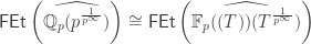
It is precisely this dearth of solid, practical connections that makes the statement of the Fontaine-Winterberger theorem (and it’s subsequent strengthenings) so mysterious, powerful, and inspiring. The Fontaine-Winterberger theorem provides an isomorphism of Galois groups. On one side we have the Galois group of something $p$ -adic, and on the other side the Galois group of something function theoretic. Less cryptically we have a continuous isomorphism

$G_{\mathbb{Q}_p(p^{\frac{1}{p^\infty}})}\cong G_{\mathbb{F}_p((T))(T^{\frac{1}{p^\infty}})}$

In fact, we have something more grand: an equivalence of (Galois) categories between the finite Galois extensions of $\widehat{\mathbb{Q}_p(p^{\frac{1}{p^\infty}})}$ and $\widehat{\mathbb{F}_p((T))(T^{\frac{1}{p^\infty}})}$ (we explain later why this gives the desired isomorphism of Galois groups). In less highfalutin language this says that we have a natural way of corresponding the finite separable extensions of $\widehat{\mathbb{Q}_p(p^{\frac{1}{p^\infty}})}$ and $\widehat{\mathbb{F}_p((T))(T^{\frac{1}{p^\infty}})}$ .

A somewhat heavy-handed way of phrasing this might be that while $\mathbb{Q}_p$ and $\mathbb{F}_p((T))$ are difficult to directly compare, once we toss in $p^{\text{th}}$ -power roots of $p$ and $T$ (which, as we attempted to argue above, play similar roles) we suddenly gain traction—a comparison is possible. In fact, we’ll be able to say that there is a direct map (only multiplicative—it obviously can’t be additive) between these $\mathbb{Q}_p(p^{\frac{1}{p^\infty}})$ and $\mathbb{F}_p((T))(T^{\frac{1}{p^\infty}})$ (or, rather their completions) which sends $p$ to $T$ . We will discuss below some reasons why these fields may seem plausible candidates for a Fontaine-Winterberger like theorem, and later still explain what we mean by the existence of an actual map sending $p$ to $T$ .

This odd comparison is part of a larger, overarching technique, the notion of tiliting, made to explicitly connect objects in the $p$ -adic world (e.g. rigid varieties) and objects in the characteristic $p$ world. This has incredible implications since, as mentioned above, many things are easier in the characteristic $p$ setting due, largely, to the existence of Frobenius. This tilting functor has its roots in the pioneering work of Fontaine (and others) in $p$ -adic Hodge theory. It was given full form by those such as Kedlaya, Liu and, Scholze. It has been an absolutely pivotal technique used in the solution to some old standing problems in arithmetic geometry, as well as the vehicle for moving towards new directions including the geometrization of the ‘arithemtic’ local Langlands conjecture.

The main goal of this post is to explain how one would naturally come to write down the tilting functor and hope that it works. Specifically, the very explicit nature of the tilting correspondence avatared by Kedlaya-Liu (whose text Foundations of $p$ -adic Hodge theory: Foundations provided me with much of the inspiration to write this post) et al. actually allows one to give an almost ‘obvious’ (of course, obvious in retrospect) sequence of ideas that naturally leads one to the creation of the tilting functor and which then fluidly necessitate precisely the properties of perfectoid fields.

Why those fields…and not others?

This subsection is largely all-for-fun fluff, and can be safely skipped or, instead, have its main content (that $G_{\mathbb{Q}_p}$ is not isomorphic to $G_{\mathbb{F}_p((T))}$ ) taken as an exercise.

Not shockingly the tilting machine is not to be operated by the easily frightened. It’s inner workings, and even technical setup, are rife with complicated definitions. In fact, a large portion of one’s first encounter with this terrifying machine is spent understanding what it even pertains to—what sort of objects can one even feed into the tilt-a-whirl?

In particular, what is it about the completions of the fields $\mathbb{Q}_p(p^{\frac{1}{p^\infty}})$ and $\mathbb{F}_p((T))(T^{\frac{1}{p^\infty}})$ that make them amenable to comparison? Why do we have to toss in large radicals of the uniformizer? This will comprise the main contents of the body of this post but, before we get there, it is worth explaining why some natural fields are not ripe for comparison.

…and not others

So, before we try and explain why the fields in the Fontaine-Winterberger are comparable in the claimed way, let us first address an important first issue. Namely, it is definitely worth mentioning explicitly that $\mathbb{Q}_p$ and $\mathbb{F}_p((T))$ are not comparable in the same way that we claim $\mathbb{Q}_p(p^{\frac{1}{p^\infty}})$ and $\mathbb{F}_p((T))(T^{\frac{1}{p^\infty}})$ are. Namely, it is not true that $G_{\mathbb{Q}_p}\cong G_{\mathbb{F}_p((T))}$ as topological groups.

There are likely many ways to see this and since this is an important point, we mention two here. One is more conceptual than the other and lends itself to natural generalization, but requires a bit of setup and some facts (albeit commonly known ones) taken on faith. We give this approach first.

Method 1

Recall that if $G$ is a profinite group, then one defines the $p$ -cohomological dimension of $G$ to be the smallest $n$ such that $H^i(G,M)=0$ for any $i>n$ and $M$ a $p$ -torsion discrete $G$ -module. We denote this number (which is possibly $\infty$ ) by $\text{cd}_p(G)$ This is obviously an invariant of topological groups. Thus, the quick answer to why $G_{\mathbb{Q}_p}$ and $G_{\mathbb{F}_p((T))}$ are not isomorphic as topological groups is that $\text{cd}_p(G_{\mathbb{Q}_p})=2$ and $\text{cd}_p(G_{\mathbb{F}_p((T))})=1$ .

The first of these is difficult to verify. Namely, it follows from local class field theory that $\text{Br}(\mathbb{Q}_p)=\mathbb{Q}/\mathbb{Z}$ so that

$H^2(G_{\mathbb{Q}_p},\mu_p)=\text{Br}(\mathbb{Q}_p)[p]=\frac{1}{p}\mathbb{Z}/\mathbb{Z}$

which shows that $\text{cd}_p(G_{\mathbb{Q}_p})\geqslant 2$ . The other inequality (which we care less about) actually is contained in the proof that $\text{Br}(\mathbb{Q}_p)=\mathbb{Q}/\mathbb{Z}$ . Essentially it comes from the fact that cohomological dimension is subadditive so that $\text{cd}_p(G_{\mathbb{Q}_p})$ is bounded by $\text{cd}_p(I_{\mathbb{Q}_p})+\text{cd}_p(\widehat{\mathbb{Z}})$ where $I_{\mathbb{Q}_p}=G_{\mathbb{Q}_p^\text{ur}}$ is the inertia group. But, this second summand is easily computed to be $1$ and the first is bounded by $1$ using the fact that every finite extension of $\mathbb{Q}_p^\text{ur}$ has trivial relative Brauer group (see Serre’s text on local fields).

Remark: The statement ‘difficult to verify’ in the previous paragraph is a bit intellectually dishonest. Namely, while proving the stated result $\text{Br}(\mathbb{Q}_p)\cong \mathbb{Q}/\mathbb{Z}$ is difficult, showing that $\text{Br}(\mathbb{Q}_p)[p]$ is non-zero is much less so. Namely, one can just construct, by hand, non-trivial $p$ -torsion elements of the Brauer group using cyclic algebras.

The second claim, that $\text{cd}_p(G_{F_p((T))})=1$ , is trivial with a bit of basic knowledge about Galois cohomology. In fact, $\text{cd}_p(G_K)\leqslant 1$ for any field $K$ of characteristic $p$ . Indeed, recall that for any field $F$ of characteristic $p$ one has that $H^i(G_F,F^\text{sep})=0$ for $i>0$ (one reason: it’s computing the cohomology of the structure sheaf on a point!). Thus, if $F$ happens to be characteristic $p$ then the Artin-Schreier sequence implies that $H^2(G_F,\mathbb{Z}/p\mathbb{Z})=0$ .

If $G$ is a pro- $p$ group one can show that one needs only check that $H^i(G,\mathbb{Z}/p\mathbb{Z})=0$ for $i>n$ to deduce that $\text{cd}_p(G)\leqslant n$ . Thus, combining these facts we see that $\text{cd}_p(G_F)\leqslant 1$ if $F$ is characteristic $p$ and $G_F$ is pro- $p$ . Finally, one uses the fact that if $G$ is any profinite group that $\text{cd}_p(G)=\text{cd}_p(H)$ for any pro- $p$ -Sylow subgroup $H$ of $G$ . Thus our group $G_K$ (where $K$ is characteristic $p$ ) satisfies $\text{cd}_p(G_K)\leqslant 1$ since it’s equal to $\text{cd}_p(H)$ for any pro- $p$ -Sylow subgroup $H$ , and $\text{cd}_p(H)\leqslant 1$ since it’s equal to $\text{cd}_p(G_F)$ for some Galois extension $F/K$ .

In some quasi-geometric sense this shows that $G_{\mathbb{F}_p((T))}$ can’t be isomorphic (as topological groups) to $G_{\mathbb{Q}_p}$ because the field $\mathbb{Q}_p$ has larger ‘size’ than $\mathbb{F}_p((T))$ or, slightly less cryptically, the site $(\mathbb{Q}_p)_{\text{f}\acute{e}\text{t}}$ is, in one measure of ‘size’, larger than $\mathbb{F}_p((T))_{\text{f}\acute{e}\text{t}}$ .

Remark: There is also some subtle foreshadowing here. Namely, the fact that $\text{cd}_p(\mathbb{Q}_p)=2$ is coming from the conributions $\text{cd}_p(I_{\mathbb{Q}_p})$ and $\text{cd}_p(G_{\mathbb{F}_p})$ (which arises as $\text{Gal}(\mathbb{Q}_p^{\text{ur}}/\mathbb{Q}_p)$ ) indicate that, somehow, to give ourselves a fighting chance of comparing characteristic $0$ and characteristic $p$ Galois groups we will either have to add a lot of ramification, or work with unramified things.

Method 2

The less conceptual, but certainly ‘simpler’ reason comes from counting number of extensions. Namely, we want to show that for some $n$ there are more Galois extensions of degree $n$ over $\mathbb{F}_p((T))$ than over $\mathbb{Q}_p$ . More specifically, there are infinitely many Galois extensions of $\mathbb{F}_p((T))$ of degree $p$ and only finitely many of degree $p$ over $\mathbb{Q}_p$ . To see this one can either use class field theory or a hodgepodge of results. Since class field theory is a bit of an overkill, we pursue the latter course of action.

One begins by recalling that the number of extensions of any fixed degree is finite over a $p$ -adic local field. The rough idea of this claim is that every extension splits as an unramified (of which there are finitely many) followed by a totally ramified extension. Thus, one only needs to explain why there are only finitely many totally ramified extensions of a $p$ -adic local field of degree $n$ . Note all such extensions come from adjoining a root of a degree $n$ Eisenstein polynomial, and conversely adjoining a root of a degree $n$ Eisenstein polynomial gives you a totally ramified Galois extension of degree $n$ . But, if $K$ is our $p$ -adic local field then the Eisenstein polynomials are in bijection with the set

$X=\mathcal{O}_K^\times\times \mathfrak{m}_K\times\cdots\times\mathfrak{m}_K\times(\mathfrak{m}_K-\mathfrak{m}_K^2)$

By Krasner’s lemma if two tuples $\overline{x}_i$ in this space are sufficiently close then the fields one obtains by adjoining the roots of the corresponding polynomials $f_i$ are the same for $i=1,2$ . Since $X$ is compact we only need finitely many such neighborhoods to cover it, and thus only finitely many extensions are obtained in this way.

To see that $\mathbb{F}_p((T))$ has infinitely many cyclic $p$ -extensions we need look no further than Artin-Schrier theory. Namely, there is a short exact sequence

$0\to \mathbb{Z}/p\mathbb{Z}\to \mathbb{F}_p((T))^{\text{sep}}\to\mathbb{F}_p((T))^{\text{sep}}\to 0$

of $G_{\mathbb{F}_p((T))}$ -modules which implies, in particular, (keeping in mind that $H^i(G_{\mathbb{F}_p((T))},\mathbb{F}_p((T))^{\text{sep}})=0$ for $i>0$ ) that

$\text{Hom}_\text{cont.}(G_{\mathbb{F}_p((T))},\mathbb{Z}/p\mathbb{Z})=H^1(G_{\mathbb{F}_p((T))},\mathbb{Z}/p\mathbb{Z})=\mathbb{F}_p((T))/(\text{im }F)$

where $F(\alpha)=\alpha^p-\alpha$ . That said, it’s obvious that this last set is infinite, which gives the desired implication.

The Witt vectors: unintentionally tilting

Important/unimportant remark: One’s head might begin to hurt in the motivation below if one imagines that $R$ is a general ring. Namely, if $R$ is such that $p\in R^\times$ then $\overline{R}:=R/pR=0$ which seems awfully strange. This is no real issue as we’ll see below, but since we will eventually restrict attention to $R$ such that $p$ is not a unit in $R$ (unless $R=0$ ) one might as well make this cognitive simplification now.

Motivation, construction, and equivalence

The story of how one might have created the tilting functor themselves starts with, not so surprisingly, the Witt vectors. These serve as a sort of baby’s-first-tilting in an idealized world of overly nice rings. Even though we shall rarely be in such an idealized world, understanding how the correspondence works there and understanding what needs to change to fix it, will lead us naturally, inexorably to a) what the tilting functor should be and b) what objects we can fruitfully hope to tilt (i.e. perfectoid objects).

So, with that highfalutin talk done with, why specifically are the Witt vectors coming up in this post? Well, in fact, for an extremely natural reason. Namely, we mentioned above that the isomorphism $G_{\mathbb{Q}_p(p^{\frac{1}{p^\infty}})}\cong G_{\mathbb{F}_p((T))(T^{\frac{1}{p^\infty}})}$ is coming, in fact, from a natural equivalence of categories

$\mathsf{FEt}\left(\widehat{\mathbb{Q}_p(p^{\frac{1}{p^\infty}})}\right)\cong \mathsf{FEt}\left(\widehat{\mathbb{F}_p((T))(T^{\frac{1}{p^\infty}})}\right)$

or, in less obtuse terms, a functorial equivalence between the finite separable extensions of $\widehat{\mathbb{Q}_p(p^{\frac{1}{p^\infty}})}$ and those of $\widehat{\mathbb{F}_p((T))(T^{\frac{1}{p^\infty}})}$ . So, really, we need a way of corresponding characteristic $0$ fields and characteristic $p$ fields in a natural way.

Now, one direction of this correspondence is fairly clear. Namely, one goes from characteristic $0$ to characteristic $p$ by first passing through some intermediary subring, and then taking a quotient by an ideal containing $p$ . For example, one can think of $\mathbb{Q}_p$ as corresponding to $\mathbb{F}_p$ by the sequence

$\mathbb{Q}_p\leadsto\mathbb{Z}_p\leadsto\mathbb{F}_p$

where the last step is taking the ring modulo $p$ . Since this first step is sort of hard to qualify for a general field (how do we choose the subring analogous to $\mathbb{Z}_p$ ?) let us focus on the second step— this is as simple as possible, it takes a ring $R$ to the ring $\overline{R}:=R/(p)$ .

So, we at least have a map from ‘characteristic $0$ like rings’ (which we make precise below) to characteristic $p$ rings (which literally just means $\mathbb{F}_p$ -algebras): take the ring modulo $p$ . But, if we are going to create a correspondence between some class of characteristic $0$ fields and some class of characteristic $p$ fields we’ll certainly need to be able to reverse this process. Namely, we want to take an $\mathbb{F}_p$ -algebra $S$ And produce from it some ‘characteristic $0$ like ring’ $R$ such that $S=\overline{R}$ . Moreover, we need this construction to be functorial and, in a perfect (pun?) world, an equivalence. One should think about the construction of the Witt vectors as being precisely this process, well, at least in the case when our $\mathbb{F}_p$ -algebra is perfect.

So, to summarize the above, the Witt vectors $W(T)$ of an $\mathbb{F}_p$ -algebras $T$ are going to be the functorial construction forming the inverse functor to the functor

$\left\{\_\_\_\_\text{`characteristic }0\text{ like rings'}\right\}\xrightarrow{R\mapsto \overline{R}}\left\{\_\_\_\_\text{ }\mathbb{F}_p\text{-algebras}\right\}$

where we’ll figure out what goes in the blanks shortly.

To help us figure out precisely what might allow us to create an equivalence in the form above, let us first start with asking what properties of our rings ‘characteristic $0$ like rings’ would be needed to make the map

$\text{Hom}(R,S)\to \text{Hom}(\overline{R},\overline{S})$

be bijective (i.e. make the reduction functor fully faithful). Let us first tackle an even simpler question. What properties of $R$ and $S$ might we need to to lift a map $\overline{R}\to\overline{S}$ to a map valued in $S_2$ where, for all $n\geqslant 0$ , we set $R_n:=R/p^nR$ and similarly for $S_n$ . The intuition being that $S_2$ is ‘closer to characteristic $0$ ‘ (and thus closer to $S$ ) than $\overline{S}=S_1$ .

So, let’s do the naive thing. Namely, if we have a map $\overline{\alpha}:\overline{R}\to\overline{S}$ then the stupidest way to get a map $\alpha_2:\overline{R}\to S_2$ is to set $\alpha_2(\overline{x})$ to be any lift of $\overline{\alpha}(\overline{x}$ ). Of course, this map is just useless—it satisfies no properties making it worthy of a ‘good’ lift. In particular, while $\alpha_2$ couldn’t be additive in general (since $S_2$ might not be an $\mathbb{F}_p$ -algebra) one might hope it to be, for example, multiplicative. So, if we seek more reasonable ways of lifting $\overline{\alpha}$ to an $\alpha_2$ we may start by analyzing better ways of lifting elements of $\overline{S}$ to $S_2$ (since, after all, any lift of $\overline{\alpha}$ will involve such liftings).

This is where the following key lemma comes into play:

Lemma 1: Let $S$ be any ring and $x,y\in S$ such that $x\equiv y\mod pR$ . Then, $x^p\equiv y^p\mod p^2 S$ .

In words that are apropos to our current struggle this says that if $z_1,z_2\in S_2$ are lifts of $\overline{y}\in \overline{S}$ then $z_1^p=z_2^p\in S_2$ .

Proof: We merely note that $x^p-y^p=(x-y)(x^{p-1}+\cdots+y^{p-1})$ . Now, mod $pR$ this second term is equivalent to $px^{p-1}$ (since mod $pR$ $x$ and $y$ are equivalent). Since $x-y$ is equivalent to $0$ modulo $pR$ this easily implies that $x^p-y^p$ is equivalent to $0$ modulo $p^2R$ as desired. $\blacksquare$

Thus, we see that choosing $p^\text{th}$ -powers of lifts can be done in a unique fashion. Unfortunately, this isn’t helpful to our situation at first glance. We are looking for methods of unique lifting, not unicity of powers of lifts. Of course, this is an easy way to remedy this. Namely, if $\overline{y}\in \overline{S}$ happens to have a unique $p^\text{th}$ -power in $\overline{S}$ , call it $\overline{y}^{\frac{1}{p}}$ , then we can take any lift of $\overline{y}^{\frac{1}{p}}$ and raise it to the $p^\text{th}$ -power. This will be a lift of $\overline{y}$ and will be independent of the lift of $\overline{y}^{\frac{1}{p}}$ by Lemma 1.

Thus, this suggests that perhaps one of the first restrictions we’d like to make on our rings $S$ is that $\overline{S}$ has unique $p^\text{th}$ -powers. We’d like to phrase this in more common mathematical parlance. Namely, if $T$ is an $\mathbb{F}_p$ -algebra then the Frobenius map is, as per usual, the ring map $\varphi:x\mapsto x^p$ . We then call an $\mathbb{F}_p$ -algebra perfect if the Frobenius map is an isomorphism. Thus, we can rephrase our first condition on $S$ by saying that we require $\overline{S}$ to be a perfect $\mathbb{F}_p$ -algebra.

We then note that this really does give us some headway in the department of lifting our map from $\overline{R}\to\overline{S}$ to a map to $S_2$ (and above). But, before we continue, let us note that while the above discussion seemed to imply that we’d want $S$ to be perfect, we really only need $R$ to be perfect since, then, the image of $R$ in $S$ (which are the only elements we’re interested in lifting) is perfect. While this level of extra generality will come in handy later, it doesn’t really change anything now—since $R$ and $S$ are both going to belong to the same category we’ll want to require that both have perfect residue rings.

Lemma 2: Let $\overline{\alpha}:\overline{R}\to\overline{S}$ be a ring map where $\overline{R}$ is perfect. Then, we obtain a multiplicative map $\alpha_n:\overline{R}\to S_n$ lifting $\overline{\alpha}$ for all $n\geqslant 1$ by sending $\overline{x}\in\overline{R}$ to $z^{p^n}$ where $z$ is any lift in $S_n$ of $\overline{\alpha}(\overline{x})$ .

So, using Lemma 2, we see that a map $\overline{\alpha}:\overline{R}\to\overline{S}$ will give rise to maps $\alpha_n:R\to S_n$ . But, our true goal is to obtain a map $\alpha:R\to S$ which, as an intermediary stage, will require a lift $\alpha_\infty:\overline{R}\to S$ . So, if we can lift to a map $\alpha_n:R\to S_n$ for all $n$ , a cheap way to obtain a lift $\alpha_\infty$ is if we knew that $S=\varprojlim S_n$ so that we can merely set $\alpha_\infty=\varprojlim\alpha_n$ . So, the next property that we might want to require is that $S$ is $p$ -adically complete.

In particular, we can refine Lemma 2 in the case that $S$ is $p$ -adically complete to:

Lemma 3: Let $\overline{R}$ be a perfect $\mathbb{F}_p$ -algebra and $S$ a $p$ -adically complete ring. Then, any ring map $\overline{\alpha}:\overline{R}\to\overline{S}$ admits a multiplicative lift $\alpha_\infty:\overline{R}\to S$ . Moreover, this lift can be defined as $\displaystyle \alpha_\infty(\overline{x})=\lim_{n\to\infty} z_n^{p^n}$ where $z_n$ is a lift of $\overline{x}^{\frac{1}{p^n}}$ .

We are very close to understanding what properties we require on $R$ and $S$ to make the reduction map be fully faithful. Finally, to finish these properties we’re going to require on $R$ (and $S$ ), we note that since our $R$ ‘s are supposed to be ‘characteristic $0$ like’ they should (at least) be $p$ -torsionless. As it turns out, these three conditions (perfect residue ring, $p$ -adically complete, and $p$ -torsionless) are actually enough to force our hand in the equivalence of categories between ‘______ characteristic $0$ like rings’ and ‘____ perfect $\mathbb{F}_p$ -algebras’.

So, to lose the baggage of excessive underscores/verbiage, let us say that a ring $R$ is a strict $p$ -ring if it’s $p$ -adically complete, $p$ -torsionless, and $\overline{R}$ is a perfect $\mathbb{F}_p$ -algebra. We think of strict $p$ -rings as being topological rings under the $p$ -adic topology. We then obtain, as we’d hope, a functor

$\left\{\text{Strict }p\text{-rings}\right\}\xrightarrow{R\mapsto \overline{R}}\left\{\text{perfect }\mathbb{F}_p\text{-algebras}\right\}$

which, at least if our intuition was solid, should be fully faithful. Then, as we said above, the Witt vector construction should be the inverse functor to the residue ring functor.

The absolutely key example to keep in mind when thinking about strict $p$ -rings is that of the $p$ -adic integers $\mathbb{Z}_p$ . They are certainly $p$ -torsionless, $p$ -adically complete, and their residue field is $\mathbb{F}_p$ a decidedly perfect $\mathbb{F}_p$ -algebra. Thus, whatever the Witt vector construction is it should have the property that $\mathbb{Z}_p=W(\mathbb{F}_p)$ .

Generalizing the case of $\mathbb{Z}_p$ we can consider $\mathbb{Z}_{p^n}$ which, by definition, is the valuation ring of the unique degree $n$ unramified extension of $\mathbb{Q}_p$ —this can be explicitly constructed as $\mathbb{Z}_p[\zeta_{p^n-1}]$ . It is certainly $p$ -adically complete and $p$ -torsionless. Moreover it’s residue field is $\mathbb{F}_{p^n}$ . Thus, we see that whatever the Witt vectors are the equality $W(\mathbb{F}_{p^n})=\mathbb{Z}_{p^n}$ will hold. Moreover, we can think of $W(\overline{\mathbb{F}_p})$ as the completion of the valuation ring $\displaystyle \bigcup_n \mathbb{Z}_p[\zeta_{p^n-1}]$ of the maximal unramified extension of $\mathbb{Q}_p$ (the valuation ring by itself is not complete!).

Remark: If these examples seems too simple, we will later have occasion to consider such beasts as $W(\mathcal{O}_{\overline{\mathbb{F}_p((T))}})$ , so if you want to see more complicated examples, just wait!

The other important example for theoretical reasons is the following. Let $\mathcal{S}$ be any set of indeterminates. Let $\mathbb{Z}[\mathcal{S}^{\frac{1}{p^\infty}}]$ be the direct limit $\varinjlim \mathbb{Z}[\mathcal{S}]$ with transition maps $\mathbb{Z}[\mathcal{S}]\to\mathbb{Z}[\mathcal{S}]$ given by sending $s\in\mathcal{S}$ to $s^p$ . Finally, let $A[\mathcal{S}]$ be the $p$ -adic completion of $\mathbb{Z}[\mathcal{S}^{\frac{1}{p^\infty}}]$ . Then, $A[\mathcal{S}]$ is $p$ -torsionless and $p$ -adically complete. It’s residue ring, the same as the residue ring of $\mathbb{Z}[\mathcal{S}^{\frac{1}{p^\infty}}]$ , is $\mathbb{F}_p[\mathcal{S}^{\frac{1}{p^\infty}}]$ (defined in a similar way) which is easily seen to be perfect. Thus, $A[\mathcal{S}]$ is a strict $p$ -ring.

Before we jump into outlining the construction of the Witt vector functor, let’s observe some nice properties about strict $p$ -rings and what they tell us about the residue ring functor (in particular, we want to show it is, in fact, fully faithful).

The first important observation is that, much like the representative example of $\mathbb{Z}_p$ , elements of a strict $p$ -ring have natural expressions as ‘power series in $p$ ‘. In fact, this property is really more a function of being $p$ -adically complete and $p$ -torsionless and what the strictness (the perfectness of the residue ring) will give us is the existence of canonical expansions.

So, to make good on our claim about $p$ -adic rings, we have the following:

Lemma 4: Let $R$ be a $p$ -adically complete $p$ -torsionless ring. For a choice of lifts $\widetilde{z}\in R$ for all $z\in \overline{R}$ every element of $R$ has a unique expansion in the form $\displaystyle \sum_{i=0}^{\infty} p^i \widetilde{z_i}$ with $z_i\in R$ for all $i$ .

Proof: Unicity follows from the fact that $R$ is $p$ -torsionless. Namely, suppose that

$\displaystyle \sum_{i=0}^\infty p^i \widetilde{z_i}=\sum_{i=0}^{\infty}\widetilde{z'_i}$

By passing to $\overline{R}$ we see that

$z_0=\widetilde{z_0}\mod pR=\widetilde{z_0'}\mod pR=z'_0$

By subtraction this implies that

$\displaystyle p\sum_{i=0}^{\infty} p^i \widetilde{z_{i+1}}=p\sum_{i=0}^\infty p^i \widetilde{z'_{i+1}}$

The fact that $R$ is $p$ -torsionless implies that

$\displaystyle \sum_{i=0}^\infty p^i \widetilde{z_{i+1}}=\sum_{i=0}^\infty\widetilde{z'_{i+1}}$

from where unicity follows by repeating the process.

For existence, let $x\in R$ . We iteratively build $z_i$ by declaring that $z_0=\overline{x}$ And $z_{i+1}=\overline{x-p^i\widetilde{z_i}}$ . It is then clear that if one considers $\displaystyle \sum_{i=0}^\infty p^i \widetilde{z_i}$ then $x$ and this sum agree modulo $p^n$ for all $n$ , and thus must be equal. $\blacksquare$

So, as stated before this lemma, if we have, instead of just a $p$ -adically complete $p$ -torsionless ring, a strict $p$ -ring then we have a natural choice of lifts $\widetilde{z_i}$ . Namely, let us note that by applying Lemma 3 to the identity map $\text{id}:\overline{R}\to\overline{R}$ we obtain a multiplicative map $[-]:\overline{R}\to R$ known as the Tecichmüller map, which, by definition has the property that $[z]\in R$ is a lift of $z\in\overline{R}$ for all $z$ . So, by Lemma 4 if $R$ is a strict $p$ -ring every element has a unique representation $\displaystyle \sum_{i=0}^\infty p^i [z_i]$ . We call the individual elements $[z]$ of $R$ Teichmüller lifts.

As an example, for $R=\mathbb{Z}_p$ we can identify the Teichmuller lifts of as precisely $0$ and the $(p-1)^\text{st}$ -roots of unity in $\mathbb{Q}_p$ . Indeed, note that since $[-]:\mathbb{F}_p\to\mathbb{Z}_p$ is multiplicative we have that $[0]=0$ and $[1]=1$ . But, also, since every element $\alpha$ of $\mathbb{F}_p$ satisfies $\alpha^p=\alpha$ the same holds for the Teichmüller lifts, which implies the claim.

So, with this setup we can finally state the key property of strict $p$ -rings that forces the reduction functor to be fully faithful:

Theorem 5: Let $R$ be a strict $p$ -ring and $S$ a $p$ -adically complete ring. Then, for any ring map $\overline{\alpha}:\overline{R}\to\overline{S}$ there exists a unique continuous ring map $\alpha:R\to S$ lifting $\overline{\alpha}$ . Specifically, if $\alpha_\infty:\overline{R}\to S$ is the multiplicative map guaranteed by Lemma 3 then

$\displaystyle \alpha\left(\sum_{i=0}^\infty p^i [z_i]\right)=\sum_{i=0}^\infty p^i \alpha_\infty(z_i)$

Proof: Tedious but straightforward calculations. See Serre’s book on local fields for proof. $\blacksquare$

Of course, we immediately obtain the following corollary:

Corollary 6: The reduction functor

$\left\{\text{Strict }p\text{-rings}\right\}\xrightarrow{R\mapsto\overline{R}}\left\{\text{Perfect }\mathbb{F}_p\text{-algebras}\right\}$

is fully faithful.

So, of course, the natural question is whether this functor is actually essentially surjective— whether it’s an equivalence of categories. The answer, as it turns out, is yes. There is actually a fairly simple proof of this fact exploiting the rings $A[\mathcal{S}]$ as before. The idea is very simple. Namely, note that every perfect $\mathbb{F}_p$ -algebra $R$ is a quotient of $\mathbb{F}_p[\mathcal{S}^{\frac{1}{p^\infty}}]$ for some $\mathcal{S}$ (in fact, you can $\mathcal{S}=R$ ). Since $A[\mathcal{S}]$ is a lift of $\mathbb{F}_p[\mathcal{S}^{\frac{1}{p^\infty}}]$ for any perfect $\mathbb{F}_p$ -algebra $\overline{R}$ we need only try to lift the ideal

$\overline{I}=\ker\left(\mathbb{F}_p[\mathcal{S}^{\frac{1}{p^\infty}}]\to\overline{R}\right)$

(for some surjection $\mathbb{F}_p[\mathcal{S}^{\frac{1}{p^\infty}}]\to \overline{R}$ ) to an ideal of $I\subseteq A[\mathcal{S}]$ and consider the strict $p$ -ring $A[\mathcal{S}]/I$ . In particular, this is easily achieved by setting

$\displaystyle I=\left\{\sum_{i=0}^\infty p^i[x_i]\in A[\mathcal{S}]:x_i\in I\text{ for all }i=0,1,\ldots\right\}$

as can be checked.

Thus, we see that the reduction functor is, in fact, an equivalence of categories. We denote the strict $p$ -ring with residue ring $T$ , if $T$ is a perfect $\mathbb{F}_p$ -algebra, as $W(T)$ and call it the ring of ( $p$ -typical) Witt vectors over $T$ .

Specific models of the Witt vectors

While the above is extremely nice, it has one serious flaw. Namely, there is the seemingly pedantic point that, as defined, $W(T)$ is really just an isomorphism class of strict $p$ -rings—it’s not a particular ring. Thankfully, there are natural ways of building a representative member of this isomorphism class which is functorial in $T$ . In other words, there are ways to actually write down a nice representation of a quasi-inverse functor to the reduction functor .

The first of these ideas is the classical one—the one from time immemorial. Namely, this is the standard process of writing down ‘universal Witt polynomials’. This approach is also useful since, as stands, we don’t really have a concrete way of describing $W(T)$ and this method certainly provides that. While we will not pursue this direct construction here (see, for example, Serre’s book on local fields) we remark as to what such a construction might look like.

This idea of buidling $W(T)$ is predicated upon the observation that we know every element of $W(T)$ looks uniquely like $\displaystyle \sum_{i=0}^\infty p^i[t_i]$ with $t_i\in S$ . Moreover, since $[-]$ is multiplicative, we know how to multiply expressions of the form $[a]\cdot[b]$ (being, of course, $[ab]$ ). The main issue then for adding or mulitplying these power series is to understand how to write $[s]+[s']$ as another ‘power series in $p$ ‘. By ‘main issue’ here, we mean that if we can describe a formula of the form

$\displaystyle [t]+[t']=\sum_{i=0}^\infty p^i[t_i]$

for $t,t'\in S$ then any multiplication/sum of elements of $W(T)$ will look like a sum of such results, and thus will be determined.

That said, this can be made seem like a much more reasonable task by noting that there have to exist universal polynomials $P_i(x,y)\in\mathbb{F}_p[x^{\frac{1}{p^\infty}},y^{\frac{1}{p^\infty}}]$ that describe such that

$[t]+[t']=\displaystyle \sum_{i=0}^\infty p^i[P_i(t,t')]$

In fact, a moment’s thought shows that if we set $\mathcal{S}=\{x,y\}$ then we can define $P_i(x,y)$ by the identity

$\displaystyle [x]+[y]=\sum_{i=0}^\infty p^i[P_i(x,y)]$

taking place in $A[\{x,y\}]$ . These polynomials are what are known as the universal Witt polynomials and one can explicitly write them down allowing one to explicitly describe $W(T)$ .

Remark: The universal Witt polynomials are somewhat complicated to write down (again, see Serre) but are part of the larger picture of the big ring of Witt polynomials over any ring $A$ which gives the set $1+t A[[T]]$ the structure of a ring (in a non-obvious way—for example, ‘addition’ is traditional multiplication). This strange object is surprisingly (to me!) deep and shows up in such varied topics as $K$ -theory to $\mathbb{F}_1$ -geometry.

There is also a more recent idea due to Cuntz and Deninger giving an extremely simple construction of an actual strict $p$ -ring with residue ring $R$ which is functorial in $R$ . Specifically, they show that if $\mathbb{Z}[R]$ is the monoid ring on the multiplicative monoid $(R,\cdot)$ and if $I$ denotes the augmentation ideal (i.e. the kernel of $\mathbb{Z}[R]\to R$ sending $\displaystyle \sum_r n_r [r]\mapsto \sum_r n_r r$ ) then the $I$ -adic completion of $\mathbb{Z}[R]$ is a strict $p$ -ring with residue ring $R$ . This is an extremely slick, functorial construction but lacks, in some sense, the incredible explicitness of the construction using Witt polynomials.

A baby ’tilting’ correspondence

We would now like to put together all of the above results to give the version of ‘idealized tilting’ that we mentioned earlier.

The first technical result we’ll need for this correspondence is the following:

Theorem 7: Let $k$ be a perfect field of characteristic $p$ . Then, $W(k)$ is a complete DVR with uniformizer $(p)$ with fraction field (denoted $B(k)$ ) a topological $\mathbb{Q}_p$ -algebra.

Proof: Let us first see that $W(k)$ is a domain. This is fairly simple though. Namely, suppose that $a,b\in W(k)$ are non-zero but $ab=0$ . Then, since $(p)$ is prime this implies that $p\mid ab$ , and so without loss of generality, we can write $pa'b=0$ with $a'=pa$ . But, since $W(k)$ is $p$ -torsionless this implies that $a'b=0$ . Repeating this process and using the fact that $\displaystyle \bigcap (p^n)=0$ implies that either $a$ or $b$ is zero.

We now claim that $W(k)$ is actually a DVR with uniformizer $(p)$ . For this it suffices to see that $W(k)$ is local since evidently $(p)$ is a maximal ideal. But, this evidently follows from the fact that $W(k)$ is $p$ -adically complete. Finally, the fact that $B(k)$ is a topological $\mathbb{Q}_p$ -algebra is clear. $\blacksquare$

From this we can give the most baby version of a correspondence between characteristic $p$ -fields and characteristic $0$ fields. Namely, let us say that a characteristic $0$ discretely valued, complete field $K$ is absolutely unramified (perhaps bad terminology—certainly non-standard) if $p$ is a uniformizer of $\mathcal{O}_K$ . A map of absolutely unramified fields is a continuous map of fields.

We then have the following:

Theorem 8: There is an equivalence of categories:

$\left\{\text{Absolutely unramified fields }K\right\}\xrightarrow{\approx}\left\{\text{Perfect characteristic }p\text{ fields }k\right\}$

given by $K\mapsto \mathcal{O}_K/(p)$ and $k\mapsto B(k):= \text{Frac}(W(k))$ .

Before we begin the proof of Theorem 8 it’s helpful to have a better understanding of continuous maps between absolutely continuous fields. The ultimate statement is the following:

Lemma 9: Let $(A,\pi,k)$ and $(A',\pi',k')$ be complete DVRs with fraction fields $K$ and $K'$ . Suppose that $\text{char}(K)=\text{char}(K')=0$ and $\text{char}(k)=\text{char}(k')=p>0$ . Then, a ring map $f:K\to K'$ is continuous if and only if $f(A)\subseteq A'$ .

Proof: Suppose first that $f$ is continuous. We then want to show that $f(a)\in A'$ if $a\in A$ . Suppose that $f(a)\notin A'$ . Then, $f(a)=(\pi')^{-n}\beta$ for some $\beta\in (A')^\times$ and some $n\geqslant 1$ . But, if $v_{\pi'}(p)=m$ this says that $f(a)=p^{-mn}\beta$ for some $\beta\in (A')^\times$ . Note then that $f(p^{mn}a)=\beta$ . If $\displaystyle \lim_{k\to\infty}(p^{mn}a)^k)=0$ then, by continuity, $\displaystyle \lim_{k\to\infty} \beta^k=0$ which is impossible since $|\beta|_{\pi'}=1$ . Thus, $\displaystyle \lim_{k\to\infty}p^{mn}a$ is not zero, which is a contradiction to $a\in A$ .

Conversely, suppose that $f(A)\subseteq A'$ . Note that $\pi\mid p$ since $\mathrm{char}(k)=p$ and similarly $\pi'\mid p$ —let’s say $p=\pi^r u$ and $p=(\pi')^{r'}u'$ . Now, if $\pi'\nmid f(\pi)$ then $f(\pi)$ is a unit in $A'$ . But, then,

$p=f(p)=f(\pi)^rf(u)$

and since $f(u)$ is a unit this implies that $p$ is a unit, which is false. Thus, we know that $v_{\pi'}(f(\pi))=n_0>0$ .

So, we now want to show that $f$ is continuous. It suffices to show, since $f$ is a ring map, that $\lim \alpha_n=0$ implies $\lim f(\alpha_n)$ . Or, equivalently, that $\lim v_\pi (\alpha_n)=\infty$ implies $\lim v_{\pi'}(f(\alpha_n))=\infty$ . But, note that $v_{\pi'}(f(\alpha_n))=n_0 v_{\pi}(\alpha_n)$ from where the conclusion follows. $\blacksquare$

Remark: I can’t shake the feeling I’ve made this woefully harder than it need be. This is just a specific version/reimagining of the statement that a map between Banach spaces(/algebras) is continuous if and only if it’s bounded. In a similar vein, it would follow easily if one would be willing to develop bare-bones language/results about Tate rings.

We can now proceed to prove Theorem 8:

Proof(Theorem 8): By Corollary 6 and Lemma 7 the Witt vectors give a fully faithful embedding

$\left\{\text{Perfect characteristic }p\text{ fields}\right\}\hookrightarrow\left\{\text{Complete DVRs}\right\}$

whose image are precisely those complete DVRs which have fraction field a $\mathbb{Q}_p$ -algebra and have $p$ as a uniformizer. In other words, those DVRs which are the valuation rings of a absolutely unramified fields.

Using Lemma 9 we deduce that $K\mapsto \text{Frac}(K)$ is an equivalence between these DVRs and absolutely unramified fields. $\blacksquare$

Theorem 8 contains in it the well-known correspondence between the unramified algebraic extensions of $\mathbb{Q}_p$ and the algebraic extensions of $\mathbb{F}_p$ .

Remark: Not shockingly, there is an exceedingly complicated way of phrasing the above constructions/theorems. Namely, if $S$ is a perfect $\mathbb{F}_p$ -algebra then its cotangent complex $\mathbb{L}_{S/\mathbb{F}_p}$ is $0$ . Indeed, the Frobenius map $\varphi:S\to S$ , being an isomorphism, induces an isomorphism $\mathbb{L}_{S/\mathbb{F}_p}\to\mathbb{L}_{S/\mathbb{F}_p}$ . But, as can be easily checked, it’s also the zero map $\mathbb{L}_{S/\mathbb{F}_p}\to \mathbb{L}_{S/\mathbb{F}_p}$ (i.e. $d(x^p)=0$ in characteristic $p$ ).

This tells us that the natural sequence of lifts

$\mathbb{Z}_p\to\cdots\to \mathbb{Z}/p^2\mathbb{Z}\to\mathbb{F}_p$

gives rise to a sequence of lifts

$S_\infty\to\cdots\to S_2\to S_1=S$

with $S_n$ a flat $\mathbb{Z}/p^n\mathbb{Z}$ -module (and $S_\infty$ a $\mathbb{Z}_p$ -module) lifting $S$ . Not shockingly,

$S_n=W_n(S):=W(S)/p^n W(S)$

and $S_\infty=W(S)=\varprojlim W_n(S)$ . This, in my opinion, hides much of the beautiful intuition gained by sussing out precisely what the content of this argument is. Namely, we are able to see why each property is completely necessary in the definition of strict $p$ -rings.

A time for reflection

Theorem 8 is precisely the type of correspondence that we hope to generalize. Of course, generalization is needed. Namely, the characteristic $0$ side of Theorem 8 involves such a small swath of fields as to not actually be extremely useful in practice. In particular, we’re interested in studying absolute Galois groups and, in every case, a base field $K$ will have extensions which are not absolutely unramified (even in the rare case that $K$ itself is absolutely unramified). Since Galois groups are, almost definitionally, groups classifying extensions, we see that this observation essentially disqualifies this correspondence for being useful in that realm.

As a particular example Theorem 8 cannot handle the extremely simple field $\mathbb{Q}_p(\sqrt{p})$ , a perfectly fine Galois extension of the absolutely unramified field $\mathbb{Q}_p$ . So, the question remains, how do we extend Theorem 8 to include these other, obvious, fields of interest—how do we include fields like $\mathbb{Q}_p(\sqrt{p})$ ? Or, more correctly, how do we adapt Theorem 8 to a class of fields closed under finite (separable) extensions?

Thus, the rest of this section will be devoted to understand how we might ‘fix’ Theorem 8, or more importantly, what sort of fields will even be amenable to a Theorem 8 type result. Specifically, we will see what sort of ‘ramified’ fields might be amenable to a correspondence between characteristic $0$ and characteristic $p$ fields. We will do this by figuring out, one by one, what properties these ‘ramified’ fields will need to possess.

The field should be normed…kind of.

This will be an exceedingly small subsection, but I think it’s helpful to separate the conditions we’d like to put on these ‘good fields’ which will help fix our Theorem 8.

So, one thing that was sort of brushed over in Theorem 8 was that it was actually a two step process. This goes back, again, to the fact that while $\mathbb{Q}_p\leadsto \mathbb{F}_p$ this is association really passes through the mediating object $\mathbb{Z}_p$ . In general, as we’ve also previously pined about, there is no canonical mediating object for a characteristic $0$ field $K$ . That said, just as in the case of absolute unramified fields we can easily fix this by putting a non-archimedean norm $|\cdot|:K\to\mathbb{R}_{>0}$ on our field. This then will allow us to naturally create the intermediary object as the valuation ring $\mathcal{O}_K=\{x\in K:|x|\leqslant 1\}$ .

Thus, the first property we will require of the class of fields we’re trying to build (which will provide a usable analogue of Theorem 8) is that they are non-archimedean fields (not precisely—see below). So, from this point forwards we are going to restrict our attention to non-archimdean fields $K$ . Having made this restriction, we can now shift focus from the field $K$ to its ring $\mathcal{O}_K$ of integral elements (which should be the object replacing the Witt vectors in Theorem 8) and figure out what properties of this ring will make them conducive to our desired form of correspondence.

This all being said, the important think about the fields we will be considering is not the norm but the topology. The reason for this is that the norm itself is a bit of a red herring. In fact, what is more important than the norm $|\cdot|:K\to \mathbb{R}_{>0}$ is the topology it generates on $K$ . Indeed, the ring $\mathcal{O}_K$ is really not a function of $|\cdot|$ itself but of this topology and, for example, if $|\cdot|':K\to\mathbb{R}_{>0}$ . To see this note that the elements of $\mathcal{O}_K$ are precisely those that are ‘power bounded’. Let me not define what this means here (I will do so in a subsequent post) but the notion of ‘boundedness’ is purely topological (at least in the setting that we’re concerned with).

Thus, while we will often times speak of normed fields $K$ we will, invariably, care more about the underlying topological field (since, again, this is really the operative thing detecting the mediating subring $\mathcal{O}_K$ ). In particular, the morphisms between the fields we care about will be continuous not isometric or bounded (although, in good situations, continuous and bounded are the same thing).

A tale of two perfections

Let us now begin our serious introspection on improving Theorem 8 by noting what the key property of fields like $\mathbb{Q}_p(\sqrt{p})$ which makes them non-amenable to study by Witt vectors. Namely, the valuation ring $\mathbb{Z}_p[\sqrt{p}]$ is certainly complete and certainly $p$ -torsionless but, what breaks down, is that $p$ is no longer a uniformizer for this complete DVR. And, why again, is this an issue for the Witt vectors? Well, the simple reason is that when we look at the residue ring $\overline{\mathbb{Z}_p[\sqrt{p}]}$ we no longer get a perfect $\mathbb{F}_p$ -algebra! Indeed,

$\overline{\mathbb{Z}_p[\sqrt{p}]}=\mathbb{F}_p[T]/(T^2)$

which is not perfect since, for example, $T^p=0$ . Thus, since Witt vectors are only able to handle perfect $\mathbb{F}_p$ -algebras we cannot attack extending Theorem 8 by directly apply them (recall, again, perfectness was needed to form canonical liftings of maps!).

So, what’s the natural thing to do? Namely, if we’re now going to want to deal with rings $R$ such that $\overline{R}$ is not perfect then, well, why not just perfect the residue ring? In particular, if we had a particularly canonical way of replacing $\overline{R}$ with a perfect $\mathbb{F}_p$ -algebra we might try to apply the Witt vectors to this algebra and use it to study $R$ . This is precisely what we do.

We come now to a somewhat funny issue. Namely, for an $\mathbb{F}_p$ -algebra $S$ there are two natural ways to try and make it perfect. These are the so-called direct perfection and inverse perfection denoted, amusingly enough, $S^{\text{perf}}$ and $S^\text{frep}$ respectively. These are characterized by either having a map from, or to, $S$ . Specifically, we have a map $S\to S^\text{perf}$ and a map $S^\text{frep}\to S$ . So, which is the correct?

Remark: I cannot claim credit for the humorous notation $R^\text{frep}$ (which conjures images of delicious icy $\mathbb{F}_p$ -beverages) it was, in fact, lifted directly from Kedlaya-Liu.

Well, as you’ll recall, the whole goal was to try and recover $R$ from $\overline{R}$ —we needed this, at least, to hope that any sort of reduction functor (relating characteristic $0$ and $p$ fields) would be fully faithful. With this in mind, what makes $\overline{R}^\text{frep}$ be the better choice is the realization that the map

$\overline{R}^\text{frep}\to\overline{R}$

induces, by Theorem 5 (since we will demand that $R$ still be $p$ -adically complete!) a map

$W(\overline{R}^\text{frep})\to R$

which, in favorable situations, will be surjective, allowing us to recover $R$ from $\overline{R}^\text{frep}$ (and, consequently, from $\overline{R}$ ). If we had chosen $\overline{R}^\text{perf}$ the direction of the arrow $\overline{R}\to\overline{R}^\text{perf}$ is in the wrong direction to apply Theorem 5 and thus there is no immediate way to connect $R$ and $W(\overline{R}^\text{perf})$ .

That said, the direct perfection will be useful for us in different ways (in particular the fact that its fundamental group doesn’t change), and thus we discuss properties of both $S^\text{perf}$ and $S^\text{frep}$ below.

So, let’s begin with the formal definitions. Namely, for an $\mathbb{F}_p$ -algebra $S$ we define the direct perfection, denoted $S^\text{perf}$ , to be

$\displaystyle \displaystyle S^\text{perf}=\varinjlim_\varphi S=\lim\left(S\xrightarrow{\varphi}S\xrightarrow{\varphi} S \to\cdots\right)$

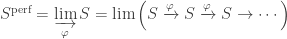
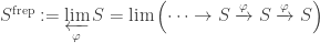
where, as per usual, $\varphi$ is the Frobenius map. We define the inverse perfection, denoted $S^\text{frep}$ , to be

$\displaystyle S^\text{frep}:=\varprojlim_\varphi S=\lim\left(\cdots\to S\xrightarrow{\varphi}S\xrightarrow{\varphi}S\right)$

These come with obvious maps $S\to S^\text{perf}$ and $S^\text{frep}\to S$ .

Remark: Of course, one can think about these two constructions by saying that $S\to S^\text{perf}$ is universal amongst maps from $S$ to perfect $\mathbb{F}_p$ -algebras and $S^\text{frep}\to S$ is universal amongst maps from perfect $\mathbb{F}_p$ -algebras to $S$ .

So, let us begin our observations about direct and inverse perfection by noting that $S^\text{perf}$ is nice in the sense that it doesn’t change the (étale) topology of $S$ in any discernible way—thus allowing one to deduce results about, say, the fundamental groups of $\mathbb{F}_p$ -algebras by the analogous results for just perfect $\mathbb{F}_p$ -algebras.

The key to this is the following:

Lemma 10: Let $S$ be an $\mathbb{F}_p$ -algebra. Then, the morphism $\text{Spec}(S^\text{perf})\to \text{Spec}(S)$ is a universal homeomorphism. More specifically, it’s radiciel (i.e. universally injective), surjective, and integral (and thus closed).

Proof: To prove the claimed results is a simple matter of checking definitions. Namely, let us begin by noting that $\text{Spec}(S^\text{perf})\to \text{Spec}(S)$ is integral. But, this is obvious—every element of the direct limit is a $p^n$ -th power of some element of $S$ .

To see it’s surjective it suffices to show that $\text{Spec}(S^\text{perf})\to\text{Spec}(S)$ is dominant (since it’s also closed by the previous paragraph). That said, the kernel of the map $S\to S^\text{perf}$ consists, evidently, of nilpotent elements of $S$ from where it follows that $\text{Spec}(S^\text{perf})\to \text{Spec}(S)$ is dominant (and thus surjective).

Finally, it remains to see why $\text{Spec}(S^\text{perf})\to \text{Spec}(S)$ is radiciel. But, by well-known results a morphism of schemes $X\to Y$ is radiciel if and only if for all $x\in X$ the morphism $k(x)\to k(f(x))$ is totally inseparable. That said, it’s easy to see that for any prime $\mathfrak{p}$ of $S$ one has that the associated map of residue fields is $k(\mathfrak{p})\to k(\mathfrak{p})^\text{perf}$ which is evidently totally inseparable. $\blacksquare$

From this we deduce the important corollary:

Corollary 11: Let $S$ be an $\mathbb{F}_p$ -algebra. Then, the map $\text{Spec}(S^\text{perf})\to\text{Spec}(S)$ induces an equivalence of sites:

$\text{Spec}(S^\text{perf})_{\acute{e}\text{t}}\cong \text{Spec}(S)_{\acute{e}\text{t}},\qquad \text{Spec}(S^\text{perf})_{\text{f}\acute{e}\text{t}}\cong\text{Spec}(S)_{\text{f}\acute{e}\text{t}}$

Also, (since the second above equivalence preserves the fiber functor) it induces isomorphism of topological groups

$\pi_1^{\acute{e}\text{t}}(\text{Spec}(S^\text{perf}))\cong\pi_1^{\acute{e}\text{t}}(S)$

As a basic example of the above we see that if $k$ is any characteristic $p$ -field, then $G_k\cong G_{k^\text{perf}}$ as topological groups. This is relevant for the Fontaine-Winterberger since it shows that $G_{\mathbb{F}_p((T))}\cong G_{\mathbb{F}_p((T))(T^{\frac{1}{p^\infty}})}$ since, as should be clear, $\mathbb{F}_p((T))(T^{\frac{1}{p^\infty}})=\mathbb{F}_p((T))^\text{perf}$ .

To discuss the relevant facts about inverse perfection, let us extend the functors of direct and inverse perfection to arbitrary rings. Namely, if $R$ is an arbitrary ring let us denote $(R/pR)^\text{frep}$ by $R^\flat$ and call it the tilt of $R$ . So, of course, if $R$ is an $\mathbb{F}_p$ -algebra then $R^\flat=R^\text{frep}$ .

Moreover, since our ultimate goal is to relate $R$ and $W(R^\flat)$ it’s helpful to give the latter a name. Namely, for any ring $R$ let us denote $W(R^\flat)$ by $A_\text{inf}(R)$ . Again, note if $R$ is $p$ -adically complete that by applying Theorem 5 to the ring map

$R^\flat\to \overline{R}$

we obtain a continuous map $\theta:A_{\inf}(R)\to R$ coming, as in Theorem 5, from a multiplicative map $\sharp:R^\flat\to R$ written exponentially (i.e. $\sharp(x)$ will be denoted $x^\sharp$ ).

Remark: The notation $A_\text{inf}(R)$ is due, I believe, to Fontaine. In his famous Periodes $p$ -adiques he shows that $A_\text{inf}(R)$ is the epaississements pro-infintesimaux universels (or ‘universal pro-infinitesimal thickening’ en Anglais) which means that, in a way one can make precise, it is the ‘universal way’ to thicken $R/pR$ to a ‘characteristic $0$ ring’ (roughly!). In other words, it is the proper replacement of the Witt vectors of $R/pR$ when $R/pR$ isn’t necessarily perfect. Specifically, it is the ‘minimal’ way to thicken our $\mathbb{F}_p$ -scheme to something $p$ -torsionless (the phrase thicken is in the same vein as the image that $\text{Spf}(\mathbb{Z}_p)$ is a pro-thickening $\varinjlim\text{Spec}(\mathbb{Z}/p^n\mathbb{Z})$ so that $\text{Spf}(\mathbb{Z}_p)$ is just a ‘really, really fat point’ whose underlying ‘physical scheme’ is $\text{Spec}(\mathbb{F}_p)$ ).

Equivalently, one can think of $A_\text{inf}(R)$ as the ring $H^0(\text{Spec}(R/pR)_\text{inf},\mathcal{O}_{\text{Spec}(R/pR)_\text{inf}})$ of global sections of the structure sheaf on the infinitesimal site $\text{Spec}(R/pR)_\text{inf}$ of $\text{Spec}(R/pR)$ .

Before we continue, let us take a moment to make the map $\sharp:A_\text{inf}(R)\to R$ explicit. Specifically,by Lemma 3 this map can be defined as $\displaystyle \sharp((x_m))=\lim_{n\to\infty}z_n^{p^n}$ where $z_n$ is a lift of the image of $(x_m)^{\frac{1}{p^n}}$ in $R/pR$ . But, note that $(x_m)^{\frac{1}{p^n}}$ is just $(x_{m+n})$ and its image in $R/pR$ is $x_n$ . Thus, we see that if we have $x=(x_n)$ then $\displaystyle x^\sharp=\lim_{n\to\infty}z_n^{p^n}$ where $z_n$ is any lift of $x_n$ . Thus, we see that the map $\theta:A_\text{inf}(R)\to R$ is given by

$\displaystyle \sum_{n=0}^\infty [(x_{n,m})]p^n\mapsto \sum_{n=0}^\infty (x_{n,m})^\sharp p^n=\sum_{n=0}^\infty \left(\lim_{m\to\infty}z_{n,m}^{p^n}\right)p^n$

where $z_{n,m}$ is a lift of $x_{n,m}\in R/pR$ to $R$ .

The two lemmas that will be important to our results are as follows:

Lemma 12: Let $R$ be a $p$ -adically complete ring. Then, there is a canonical isomorphism of multiplicative monoids

$\displaystyle R^\flat\cong \lim_{x\mapsto x^p}R$

given by

$\underline{x}\mapsto \left(\underline{x}^{\sharp},\left(\underline{x}^{\frac{1}{p}}\right)^\sharp,\ldots\right)$ .

Proof: This is largely a matter of unpacking the definitions.

By definition, the map $R^\flat\to \overline{R}$ takes a tuple $\underline{x}=(x_0,\ldots,)$ in $R^\flat$ to $x_0\in\overline{R}$ . So, to lift this to a map $R/p^n R$ we first take the $p^n$ -th root of $\underline{x}$ in $R^\flat$ . This is given explicitly by $(x_n,\ldots)$ (shifting $n$ to the left). We then look at its image under $R^\flat\to R$ , which is $x_n$ . We then choose a lift $z$ of it in $R/p^n R$ and consider $z^{p^n}$ . Thus, if we think of elements of $R$ as tuples (i.e. identify an element $r\in R$ with $(r\mod p,r\mod p^2,\ldots)$ we have that $([\underline{x}])^\sharp$ is given by $(t_{1,1},\ldots)$ with $t_{1,i}=z_{1,i}^{p^i}$ where $z_{1,i}$ is a lift of $x_{i-1}$ to $R/p^i R$ .

Now, $\underline{x}^{\frac{1}{p}}=(x_1,\ldots)$ and thus we can describe $\left(\underline{x}^{\frac{1}{p}}\right)^\sharp$ as $(t_{2,1},\ldots)$ with $t_{2,i}=z_{2,i}^{p^i}$ where $z_{2,i}$ is a lift of $x_{i}$ . Thus, in general, we can describe $\left(\left[\underline{x}^{\frac{1}{p^m}}\right]\right)^\sharp$ as $(t_{m,1},\ldots)$ with $t_{m,i}=z_{m,i}^{p^i}$ where $z_{m,i}$ is a lift of $x_{i+m-2}$ .

So, let us verify that $(t_{m,i})$ , as an element of $\displaystyle R^{\oplus\mathbb{N}}$ , is really in $\displaystyle \varprojlim_{x\mapsto x^p} R$ . Indeed, we need that check that for all $m\geqslant 1$ we hvae that $(t_{m+1,i})^p=(t_{m,i})$ . But, this amounts to the statement that $t_{m+1,i}^p=t_{m,i}$ . But, retracing, we see that $t_{m+1,i}=z_{m+1,i}^{p^i}$ where $z_{m+1,i}$ is a lift of $x_{i+m-1}$ and $t_{m,i}=z_{m,i}^{p^i}$ where $z_{m,i}$ is a lift of $x_{i+m-2}$ . Thus, we need to check that $z_{m+1,i}^{p^{i+1}}=z_{m,i}^{p^i}$ but, by Lemma 1, it suffices to check that $x_{m+i-1}^p=x_{m+i-2}$ which, of course, was by design.

So, we’ve verified that our map actually sends $R^\flat$ into $\displaystyle \varprojlim_{x\mapsto x^p}R$ . Moreover, it’s clearly multiplicative since the map $R^\flat\to R$ was multiplicative. Thus, it remains to show bijectivity.

But, this is clear. Namely, the above arduous unraveling of definitions shows that we can, in fact, write down the inverse. Namely, it takes a tuple $(t_{m,i})$ in $\displaystyle\varprojlim_{x\mapsto x^p}R$ to the tuple in $R^\flat$ given by $(t_{m,1})$ (i.e. reducing mod $p$ ). $\blacksquare$

Remark: In a way that will (hopefully) in a later post be made clear, it’s really better to define $R^\flat$ by $\displaystyle \varprojlim_{x\mapsto x^p} R$ , in which case the sharp map $\sharp:R^\flat\to R$ is just projection onto the first $R$ factors. While this is certainly ‘simpler’ than the sharp map defined above, it’s really just hiding the difficulties in the definition since, ultimately, one will want to relate $\displaystyle (R/pR)^\text{frep}$ which will necessitate one to deal with the sharp map as we’ve defined it.

From this, we obtain the following ostensibly non-obvious corollary:

Corollary 13: If $R$ is an integral domain, then so is $R^\flat$ .

We can, in fact, extend to Lemma 12 to actually obtain the structure of $R^\flat$ , as a ring, in terms of the monoid $\displaystyle \varprojlim_{x\mapsto x^p}R$ . In particular, from Lemma 12 we can describe what the addition on $\displaystyle \varprojlim_{x\mapsto x^p}R$ , the one in inherited from its identification with $R^\flat$ , is in simple terms.

Lemma 14: Let $R$ be a $p$ -adically complete ring. Then, under the isomorphism of monoids

$\displaystyle R^\flat\to \varprojlim_{x\mapsto x^p}R$

the addition on $\displaystyle \varprojlim_{x\mapsto x^p}R$ by transfer of structure is given as follows:

$(x_i)+(y_i)=(z_i)$

with

$\displaystyle z_i=\lim_{n\to\infty}(x_{i+n}+y_{i+n})^{p^n}$

Proof: This is not too difficult, and is a good bracing exercise to make sure one understands the definitions of the objects involved. $\blacksquare$

The other substantial result that we’ll need is a condition on when $\theta:A_{\inf} (R)\to R$ is surjective:

Lemma 15: Let $R$ be a $p$ -adically complete ring. Then, $\theta:A_{\inf} (R)\to R$ is surjective if and only if $\overline{R}$ is semiperfect.

An $\mathbb{F}_p$ -algebra $R$ is called semiperfect if Frobenius is surjective (perhaps not injective!).

Proof: Suppose that $\theta$ is surjective. Then, of course, the map we get by reducing modulo $p$ is surjective. In other words, the map $R^\flat\to \overline{R}$ is surjective. But, this says precisely that $\overline{R}^\text{frep}\to\overline{R}$ is surjective. Since this sends $(x_0,\ldots)$ to $x_0$ this says precisely that $\overline{R}$ is semiperfect.

Conversely, if $\overline{R}$ is semiperfect then $R^\flat\to\overline{R}$ is surjective. Now every element of $R$ can be written (possibly non-uniquely) as $\displaystyle \sum_{i=0}^\infty p^i z_i$ where the $z_i$ can be taken to live in a fixed set of lifts of elements from $\overline{R}$ . Since the map $\displaystyle \theta$ takes $\displaystyle \sum_{i=0}^\infty p^i[\underline{x}_i]$ to $\displaystyle \sum_{i=0}^\infty p^i [\underline{x}_i^\sharp]$ . Thus, it’s clear that $\theta$ is surjective if we can show that the set $\sharp((x_n))$ forms a set of lifts of elements of $R/pR$ . That said, note that $\sharp((x_n))\mod p$ is just $x_0\mod p$ . Thus, again, we only need that every element of $R/pR$ shows up as the first term of a sequence in $R^\flat$ which is equivalent to $R/pR$ being semi-perfect. $\blacksquare$

From this section we can deduce two properties of our field $K$ , or more operatively its ring of integers $\mathcal{O}_K$ , that will make them amenable to recovery from the ring $\mathcal{O}_K/p\mathcal{O}_K$ . Namely, Lemma 15 tells us that we will be able to recover $\mathcal{O}_K$ from $A_\text{inf}(\mathcal{O}_K)$ (or, equivalently, from $\mathcal{O}_K/p\mathcal{O}_K$ ) as soon as $\mathcal{O}_K$ is $p$ -adically complete and $\mathcal{O}_K/p\mathcal{O}_K$ is semi-perfect. Thus, besides wanting $K$ to be a non-archimedean field (or, again, a topological field with topology coming from a non-archimedean norm), we’re going to want to declare that these two properties of $\mathcal{O}_K$ hold.

Eliminating absolute unramified fields

So far we have figured out that to effectively rework Theorem 8 to a usable (from a Galois group perspective) state we should focus on non-archimedean fields $K$ such that $\mathcal{O}_K$ is complete and has semi-perfect residue ring. We are extremely close to nailing down precisely the type of fields that will be of interest to us but, as of now, we can’t hope to have a complete correspondence between fields with these properties and characteristic $p$ fields.

The reason being, roughly, we have essentially (by demanding our fields $K$ satisfy these above properties) pinned down either ‘very ramified’ or ‘very unramified’ extensions of $\mathbb{Q}_p$ and, as Theorem 8 showed us, it is not the latter that we want to consider. To explain this relatively cryptic statement, consider an algebraic extension $K/\mathbb{Q}_p$ . Then, one can fairly easily show that $\widehat{K}$ (the completion of $K$ with respect to its specified norm) will satisfy the properties listed above (a complete non-archimedean field with semi-perfect residue ring) only if $K/\mathbb{Q}_p$ is either unramified or infinitely ramified.

Indeed, if $K/\mathbb{Q}_p$ is unramified, then evidently it satisfies all of the criteria. Suppose then that $K/\mathbb{Q}_p$ is not unramified and let $K_0\subseteq K$ be the largest unramified subextension. If $K/\mathbb{Q}_p$ is not infinitely ramified then $K/K_0$ is finite and $K$ discretely valued. Note then that if $[K:K_0]=n$ then one can see that $\mathcal{O}_K/(p)$ can’t be semi-perfect. Indeed, let $\pi$ be a uniformizer of $K$ and suppose that $\overline{\pi}\in\mathcal{O}_K/(p)$ has a $p^\text{th}$ -root. Then, there exists $\beta\in \mathcal{O}_K$ such that $\beta^p=\pi+p\alpha$ for some $\alpha\in \mathcal{O}_K$ . This then implies that $|\beta|^p=|\pi|$ (since $|\pi|>|p\alpha|$ ) which contradicts that $\pi$ is a uniformizer.

Thus, to eliminate these unramified fields from the equation (so as to not repeat the inadequacies of Theorem 8—specifically, to obtain a class of fields closed under finite separable extensions) we need to impose one last condition on our non-archimedean field $K$ which, intuitively, captures ‘unramifiedness’ (thus eliminating the absolute unramified fields). One can see quite clearly from the above argument that the key thing about being finitely ramified which broke semi-perfectness was non-discreteness of the valuation. This non-discreteness also quite neatly eliminates the absolutely unramified extensions of Theorem 8. Thus, the last condition we will need to pare down our fields to a set amenable to Theorem 8 type results (which, this time, will be usable in the study of Galois groups) will be to require that the absolute value on $K$ is non-discrete.

Remark: Again, note that this is really a topological property. Namely, one can tell from the underlying topological field $K$ whether a normed field is discrete. This is because one can get a handle on the maximal ideal of $\mathcal{O}_K$ as the set of topologically nilpotent elements (i.e. elements $x$ such that $\displaystyle \lim_{n\to\infty}x^n=0$ ).

The definition…finally

After all of this reflection, we come to a similar situation when intuiting the definition of strict $p$ -rings. Namely, whatever this closed-under-finite-extension class of fields which will be amenable to Theorem 8 type results is, it should probably possess (by our analysis above) the following properties: it’s a complete non-archimedean field with non-discrete absolute value and which has (ring of integers with) semi-perfect residue ring.

Remark: Note that we really intuited in our discussion of $A_\text{inf}$ that our field $K$ should have the property that $\mathcal{O}_K$ is $p$ -adically complete and has semi-perfect residue ring. That said, note that $\mathcal{O}_K$ being $p$ -adically complete and $K$ having complete absolute value are essentially the same—at least in characteristic $0$ .

Thus, without further adieu, let us combine all of these features together and make our lives much easier by eliminating this adjectival clutter. Namely, let us define a complete non-archimedean field $K$ to be perfectoid if it is non-discrete and $\mathcal{O}_K/\mathfrak{p}$ is semi-perfect. The rest of this post will then be devoted to showing that we can, for perfectoid fields, create a useful analogue of Theorem 8 which will allow us to compare Galois groups in characteristic $0$ and characteristic $p$ (or, more to the point, correspond fields in characteristic $0$ and characteristic $p$ ).

Perfectoid fields and their tilts

Before we jump into actually creating the analogy of Theorem 8 for perfectoid fields, it will be first helpful to understand some basic properties of these objects.

Tilting preserves perfectoidness

Our first step towards an earnest study of perfectoid fields, and whatever sort of characteristic $0$ /characteristic $p$ correspondence they yield, will begin by studying how perfectoid fields behave under tilt. In particular, one of the key results that we will need is that, in fact, the tilt of a perfectoid field is still perfectoid. Of course, this is technically not a well-posed statement since perfectoid fields are normed fields (i.e. they have a topology coming from a norm!) and, until this point, tilting has only produced algebraic objects with no sort of analytic accouterments. Thus, the content of this section will be showing that, in fact, if $K$ is a perfectoid field then its tilt comes with a natural norm (once we’ve fixed a norm upstairs) making the associated topological field a perfectoid field.

So, before we seriously begin, let us make a quick notational pit stop. Namely, if $K$ is a perfectoid field then $\mathcal{O}_K^\flat$ is a domain (by Corollary 13) and we’d like to give symbol to the associated field $\text{Frac}(\mathcal{O}_{K^\flat})$ . Following standard notational convention we will denote this field by $K^\flat$ despite the unfortunate clash with our already defined notation: namely, $K^\flat$ does not mean $(K/pK)^\text{frep}$ . We apologize for this confusion but, in all reality, it will always be clear from context which notion of $\flat$ is meant. So, with this all being said, we can summarize the previous paragraph by saying that our main goal this section is to supply $K^\flat$ with a natural norm $|\cdot|_\flat$ built, somehow, from the norm $|\cdot|$ on $K$ and show that $K^\flat$ with $|\cdot|_\flat$ is perfectoid.

To define $|\cdot|_\flat$ we will essentially import the absolute value $|\cdot|$ from $K$ via the map $\sharp$ . Namely, let us first define $|\cdot|_\flat:\mathcal{O}_{K^\flat}\to\mathbb{R}_{>0}$ by declaring:

$|x|_\flat:=|x^\sharp|$

Let us quickly verify that this is a norm on $\mathcal{O}_K^\flat$ . It’s clearly multiplicative since $\sharp$ and $|\cdot|$ are. Moreover, it’s clear that $|0|=0$ and $|1|$ . Thus, it remains to show that $|\cdot|_\flat$ satisfies the strong triangle inequality

$|(x_n)+(y_n)|_\flat\leqslant\max\{|(x_n)|_\flat,|(y_n)|_\flat\}$

To see this, choose lifts $\widetilde{x_n}$ of $x_n$ and $\widetilde{y_n}$ of $y_n$ in $R$ . Then, note that $\widetilde{z_n}:=\widetilde{x}_n+\widetilde{y_n}$ is a lift of $x_n+y_n$ . So

$\begin{aligned}|(x_n)+(y_n)|_\flat &= \left|\left((x_n)+(y_n)\right)^\sharp\right|\\ &= \left|\lim_{n\to\infty}\widetilde{z}_n^{p^n}\right|\\ &= \lim_{n\to\infty}\left|\widetilde{z}_n\right|^{p^n}\\ &= \lim_{n\to\infty}\left|\widetilde{x_n}+\widetilde{y_n}\right|^{p^n}\\ & \leqslant \lim_{n\to\infty} \max\{|\widetilde{x_n}|,|\widetilde{y_n}|\}^{p^n}\\ &= \max\left\{\left|\lim_{n\to\infty}\widetilde{x_n}^{p^n}\right|,\left|\lim_{n\to\infty}\widetilde{y_n}^{p^n}\right|\right\}\\ &= \max\left\{|(x_n)^\sharp|,|(y_n)^\sharp|\right\}\\ &= \max\left\{|(x_n)|_\flat,|(y_n)|_\flat\right\}\end{aligned}$

thus verifying that, in fact, $|\cdot|$ is an absolute value on $\mathcal{O}_K^\flat$ .

Another useful fact to observe about $|\cdot|_\flat$ is how one can use lifts of a tuple $(x_i)\in R^\flat$ to compute it. Namely, suppose that $(x_i)=(x_0,\ldots)\in R^\flat$ and choose lifts $z_i\in R$ of each $x_i$ . Then, the following equality holds for all $m$ :

$\max\{|(x_i)|_\flat,|p|^m\}=\max\{\left|z_m^{p^m}\right|,|p|^m\}$

In particular, we see that if $m\gg 0$ then $|(x_i)|_\flat=|z_m|^{p^m}$ . This equality can be verified quite easily by hand.

Since $\mathcal{O}_K^\flat$ is a domain we can extend $|\cdot|_\flat$ to a rank $1$ valuation on $K^\flat$ . We claim that, in fact, $\mathcal{O}_K^\flat$ is the valuation ring of this rank $1$ valuation.

So, let us prove this claim:

Lemma 16: The ring $\mathcal{O}_K^\flat$ is the valuation ring for $|\cdot|_\flat$ on $K^\flat$ . Thus, $\mathcal{O}_{K^\flat}=\mathcal{O}_K^\flat$ .

Proof: It suffices that for $x,y\in\mathcal{O}_K^\flat$ one has that $x\mid y$ if and only if $|x|_\flat\leqslant |y|_\flat$ . It’s clear that if divisibility happens, then inequality happens. The converse is a standard argument by choosing lifts of $x$ and $y$ to $\mathcal{O}_K$ and showing that since the limits of these lifts have the desired inequality of norms, one can build an element realizing the division. $\blacksquare$

Thus, we see that if $K$ is a non-archimedean field with rank $1$ -valuation $|\cdot|$ then $K^\flat$ is a non-archimedean field with rank $1$ -valuation $|\cdot|_\flat$ . Moreover, it’s obvious that if $K$ is complete, then so is $K^\flat$ . Indeed, any Cauchy sequence of elements in $\mathcal{O}_{K^\flat}$ must have terms which eventually stabilize, which gives the result.

So, we see that $K^\flat$ is a complete non-archimedean field. Moreover, note that $\mathcal{O}_{K^\flat}/(p)$ is just $\mathcal{O}_{K^\flat}$ but, since $\mathcal{O}_{K^\flat}=\mathcal{O}_K^\flat$ we know then that $\mathcal{O}_{K^\flat}$ is perfect and consequently semi-perfect. Thus, the only impediment to us gleefully exclaiming that $K^\flat$ is perfectoid is the possible issue that $|\cdot|_\flat$ might be non-discrete.

That said, we can actually do one better than just showing non-discreteness:

Lemma 17: Let $K$ be a non-discrete valued field such that $\mathcal{O}_K$ has semiperfect residue ring and is complete. Then, $|K^\times|=\left|(K^\flat)^\times\right|_\flat$ . Moreover, the topology on $\mathcal{O}_{K^\flat}$ induced by this norm agrees with the inverse limit topology on $\mathcal{O}_K^\flat$ by giving each of the $\mathcal{O}_K/p\mathcal{O}_K$ the discrete topology.

Proof: So, let us begin by noticing that by the equality

$\max\{|(x_i)|_\flat,|p|^m\}=\max\{|z_m|^{p^m},|p|^m\}$

that $|(K^\flat)^\times|_\flat\cap (|p|,1)=|K^\times|\cap(|p|,1)$ . In fact, evidently $|(K^\flat)^\times|\subseteq |K^\times|$ (by construction), and thus we need only check that if $\xi \in |K^\times|\cap (|p|,1)$ it should be in $|(K^\flat)^\times|$ . So, choose $z_0\in\mathcal{O}_K$ with $|z_0|=\xi$ . Since $\mathcal{O}_K/p\mathcal{O}_K$ is semiperfect we know that we can find some tuple $(x_i)\in\mathcal{O}_{K^\flat}$ such that $x_0=z_0\mod p\mathcal{O}_K$ . Note then that for $m$ sufficiently large we have that

$|(x_i)|_\flat=\max\{|(x_i)|_\flat,|p|^m\}=\max\{|z_m|^{p^m},|p|^m\}=|z_m|^{p^m}$

that said, we know that

$z_m^{p^m}=z_0+pu$

and so, by taking norms, recalling that $|z_0|>|p|$ we see that

$|(x_i)|_\flat=|z_m|^{p^m}=|z_0|$

as desired.

While this doesn’t imply, for arbitrary $K$ and $K^\flat$ , that $|K^\times|=|(K^\flat)^\times|$ , it does for $K$ perfectoid since one can use the discreteness of $K$ and the perfectness of $K^\flat$ (see Theorem 20, which is independent of this result) to move the argument to the range $(|p|,1)$ .

We leave the second claim to the reader. $\blacksquare$

Thus, since $|\cdot|$ is non-discrete, we deduce the following:

Theorem 18: Let $(K,|\cdot|)$ be a perfectoid field. Then, $(K^\flat,|\cdot|^\flat)$ is a perfectoid field.

Note, moreover, that the association $(K,|\cdot|)\mapsto (K^\flat,|\cdot|_\flat)$ defines a functor from perfectoid fields to perfectoid fields in characteristic $p$ where, in both cases, the morphisms we are interested in are just continuous morphisms.

Basic properties of perfectoid fields

Let us now enumerate the basic properties of perfectoid fields and their tilts which were precisely the guiding motivation for their definition:

Theorem 19: Let $K$ be a perfectoid field with tilt $K^\flat$ . Then:

$K^\flat$ is a characteristic $p$ perfectoid field.

$|K^\times|=|(K^\flat)^\times|_\flat$ .

$\mathcal{O}_{K^\flat}=\mathcal{O}_K^\flat\to\mathcal{O}_K/p\mathcal{O}_K$ is surjective with kernel $(z)$ where $z$ is any element of $\mathcal{O}_{K^\flat}$ with $|z|_\flat=|p|$ .

There is a natural isomorphism $\kappa_K\cong \kappa_{K^\flat}$ where the kappa notation denotes residue field.

The map $A_{\text{inf}}(\mathcal{O}_K)\to \mathcal{O}_K$ is surjective.

Proof: Properties 1. and 2. have already been discussed.

The fact that $\mathcal{O}_{K^\flat}\to\mathcal{O}_K/p\mathcal{O}_K$ is surjective follows from the fact that $\mathcal{O}_K$ is assumed to have semi-perfect residue field. Now, to show the claim that the kernel is generated by $(z)$ for any $z$ with $|z|=|p|$ we really just need to show that $\alpha$ is in the kernel of the map $\mathcal{O}_{K^\flat}\to \mathcal{O}_K/p\mathcal{O}_K$ if and only if $|\alpha|_\flat\leqslant |p|$ . Now, if we write $\alpha=(x_i)$ and if $z_i\in\mathcal{O}_K$ is a lift of $x_i$ then we know that $\alpha^\sharp\in\mathcal{O}_K$ is just the element of $\displaystyle \varprojlim \mathcal{O}_K/p^n\mathcal{O}_K$ given by the tuple $(z_i^{p^i}+p^i\mathcal{O}_K)$ . Moreover, we know that $|\alpha|_\flat=|\alpha^\sharp|$ and thus it suffices to show that $\alpha$ is in the kernel of this map if and only if $|\alpha^\flat)|\leqslant |p|$ .

That said, note that for all $i\geqslant 1$ we have that

$\theta(\alpha)-z_i^{p^i}=p^i a$

for some $a\in\mathcal{O}_K$ . So, suppose that $\alpha$ is in the kernel of the discussed map. Then, for all $i$ we have that $z_i^{p^i}\in p\mathcal{O}_K$ . Thus, we see that $\alpha^\sharp$ is divisible by $p$ and thus $|\alpha^\sharp|\leqslant |p|$ . Conversely, if $|\alpha^\sharp|\leqslant p$ then evidently $z_i^{p^i}$ is divisible by $p$ for all $i$ which implies the result.

To prove 4., let us note that we have ring isomorphisms

$\mathcal{O}_{K^\flat}/(z)\cong \mathcal{O}_K/p\mathcal{O}_K$

with $|z|_\flat=|p|$ . But, we then get a natural isomorphism between the maximal reduced quotients of these rings which are naturally $\kappa_{K^\flat}$ and $\kappa_K$ respectively.

Property 5 follows, again, from Lemma 15. $\blacksquare$

We also make the following trivial observation about what perfectoid fields in characteristic $p$ look like:

Theorem 20: Let $K$ be a valued field of characteristic $p$ . Then, $K$ is perfectoid if and only if $K$ is complete, non-discretely valued, and perfect. Moreover, in this case, there is a natural isomorphism $K^\flat\cong K$ .

Proof: Obvious. Namely, the only condition left to check is that $\mathcal{O}_K/p\mathcal{O}_K=\mathcal{O}_K$ is semi-perfect which is equivalent to $K$ being semi-perfect (since $\mathcal{O}_K$ is integrally closed), but this is equivalent to $K$ being perfect (since it’s a field). The second claim is clear. $\blacksquare$

This justifies the moniker perfectoid since they are generalizations of perfect which work in both characteristic $p$ and characteristic $0$ .

Examples

Let us end this section by giving some instructive examples/non-examples of perfectoid fields and their tilts:

Example 1: Let $K$ be the completion of $\mathbb{Q}_p(\zeta_{p^\infty})$ . We claim that $K$ is perfectoid. It’s evidently complete and non-discrete so it remains to see why it has semi-perfect residue ring. That said, note that $\mathcal{O}_K$ is the same thing as the completion of $\mathbb{Z}_p[\zeta_{p^\infty}]$ which is the same as the $p$ -adic completion of this ring. Thus, it’s easy to see that the residue ring of $\mathcal{O}_K$ is the same thing as the residue ring of $\mathbb{Z}_p[\zeta_{p^\infty}]$ .

So, let us compute what the residue ring of $\mathbb{Z}_p[\zeta_{p^\infty}]$ . But, it’s not hard to see that this is just the ring $\mathbb{F}_p[T_1,\ldots]/I$ where $I=(1+T_1+\cdots+T_1^{p-1},T_2^p-T_1,T_3^p-T_2,\ldots)$ . To see that this is semi-perfect we really only need to check that the generators are $p^\text{th}$ -powers, but this is manifestly true.

One can then check that $\mathcal{O}_K^\flat$ is precisely $\mathbb{F}_p((T^{\frac{1}{p^\infty}}))$ which, by definition, is the $T$ -adic completion of $\mathbb{F}_p((T_1))(T_1^{\frac{1}{p^\infty}})$ —the element $T$ can be thought of explicitly as the sequence $(T_1,T_2,T_3,\ldots)$ . The verification of this is not overly difficult, and left to the reader.

Example 2: Let $K$ be the completion of $\mathbb{Q}_p(p^{\frac{1}{p^\infty}})$ . We claim that $K$ is perfectoid. Indeed, it’s, as in the previous example, obviously complete and non-discrete, so it suffices to see that its ring of integers has semi-perfect residue ring. And, again as in the last example, it suffices to see that $\mathbb{Z}_p[p^{\frac{1}{p^\infty}}]$ has semi-perfect residue ring.

But, again, here, there is a very nice description of the residue ring. Namely, it’s just $\mathbb{F}_p[T_1,\ldots,]/J$ where $J=(T_1^p,T_2^p-T_1,\ldots)$ . One can, in fact, see that this $\mathbb{F}_p$ -algebra is isomorphic to the residue ring of Example 1 by sending $T_1\mapsto 1+T_1$ . The point being, that while $\zeta_p$ and $p^{\frac{1}{p}}$ differ hugely in characteristic $0$ , when moving to characteristic $p$ they become ‘something whose $p^\text{th}$ power is $0$ freely’ and ‘something whose $p^{\text{th}}$ power is $1$ freely’, which are easily moved between each other by adding 1. Thus, again, we see that in this example $K^\flat\cong \mathbb{F}_p((T^{\frac{1}{p^\infty}}))$ .

This example, of course, is what will underlie the Fontaine-Winterberger isomorphism. Note, moreover, that as promised the correspondence $\widehat{\mathbb{Q}_p(p^{\frac{1}{p^\infty}})}\leadsto \mathbb{F}_p((T^{\frac{1}{p^\infty}}))$ actually has $T$ corresponding to $p$ . Or, more correctly, we observe that $T^\sharp=p^{\frac{1}{p}}$ ! Thus, we have created a ‘correspondence’ (we have yet to justify that word) which, in some sense, ‘carries $T$ to $p$ ‘.

Example 3: Let $K=\mathbb{C}_p$ , then $K$ is perfectoid. Indeed, note that $\mathbb{C}_p$ is certainly non-discrete (it’s value group is $p^{\mathbb{Q}}$ ) and complete, thus it remains to see why it’s residue ring is semi-perfect. But, this is clear since $\mathcal{O}_{\mathbb{C}_p}$ has $p^\text{th}$ -roots (since $\mathbb{C}_p$ is algebraically closed and $\mathcal{O}_{\mathbb{C}_p}$ integrally closed).

Let us now begin to compute $K^\flat$ . This will actually be somewhat difficult. So, we give an outline here of why this is true, leaving some of the details for later. Namely, we claim that it is $\widehat{\overline{\mathbb{F}_p((T))}}$ . To see this, we will later show that since $\overline{\mathbb{Q}_p}$ is algebraic over $\mathbb{Q}_p(p^{\frac{1}{p^\infty}})$ , as considered in Example 3, that $\mathbb{C}_p^\flat$ will be algebraic over $\mathbb{F}_p((T^{\frac{1}{p^\infty}}))=K^\flat$ showing that it is a complete subfield of $\widehat{\overline{\mathbb{F}_p((T))}}$ . But, as we will later see, since $\mathbb{C}_p$ is closed the same is true for $\mathbb{C}_p^\flat$ . Thus, $\mathbb{C}_p^\flat$ is algebraic over $\widehat{\mathbb{F}_p((T^{\frac{1}{p^\infty}}))}$ , algebraically closed, and complete, which implies that it’s isomorphic to $\widehat{\overline{\mathbb{F}_p((T))}}$ as claimed.

Example 4: Example 1 tips us off as to how to create many perfectoid fields. Namely, note that $\mathbb{Q}_p(\zeta_{p^\infty})$ is just the Lubin-Tate extension/tower of $\mathbb{Q}_p$ corresponding to the uniformizer $p$ . More generally, if $K$ is any $p$ -adic local field and $\pi\in K$ is any uniformizer, then the Lubin-Tate extension $K_\pi/K$ will have the property that $\widehat{K_\pi}$ is perfectoid.

Example 5: A major source of examples of perfectoid fields, coming from the work of Winterberger, Fontaine et al., are the so-called arithmetically profinite (APF) extensions of a $p$ -adic local field $K$ . They are, according to the forementioned people, known to have perfectoid completions. We will not define APF here but, suffice it to say, knowing that $L/K$ such that $\text{Gal}(L/K)$ a $p$ -adic Lie group implies that $L/K$ is APF. The example in 4 was of this type since $\text{Gal}(K_\pi/K)\cong\mathcal{O}_K^\times$ (as is the point of Lubin-Tate extensions) and $\mathcal{O}_K^\times$ is a $p$ -adic Lie group.

Inverting the tilting functor

Technical results

Now that we have begun to get a handle on what the tilting functor actually looks like for perfectoid fields, we can understand what aspect of perfectoid fields allow us actually sucessfully create a correspondence between characteristic $0$ and characteristic $p$ fields. Specifically, we would like to ‘invert’ the tilting functor to create some sort of correspondence of the form

$\left\{\begin{matrix} \text{Perfectoid fields of}\\ \text{characteristic }0\end{matrix}\right\}\xrightarrow{\approx}\left\{\begin{matrix}\text{Perfectoid fields of}\\ \text{characteristic }p\end{matrix}\right\}:K\mapsto K^\flat$

which will be useful for making the sort of Galois group comparisions as in the Fontaine-Winterberger theorem. Of course, this cannot literally work! We’ve already observed in Example 1 and Example 2 above that two non-isomorphic perfectoid fields of characteristic $0$ give the same tilt. We can fix the above by considering perfectoid extensions of a fixed perfectoid field $K$ and extensions of its tilt $K^\flat$ . In particular, in a way in which we’ll soon make precise, the ambiguity which exists in ‘untilting’ extensions of $K^\flat$ is eliminated once we fix the ‘untilt’ $K$ of $K^\flat$ .

But, before we get to this level of detail, it’s extremely helpful to not make restrictions about lying over some fixed base field. Namely, even though the literal tilting functor (with no restrictions on base) is demonstrably not an equivalence, one might ask what sort of extra data is contained in $K$ beyond $K^\flat$ —what extra statistic of the completions of $\mathbb{Q}_p(p^{\frac{1}{p^\infty}})$ and $\mathbb{Q}_p(\zeta_{p^\infty})$ is needed to distinguish them beyond knowing they have the same tilt?

Remark: Scholze has said that he views the tilting operation as being analogous to the underlying-space functor sending a complex analytic space $X$ to its underlying topological space $|X|$ . The justification for this point of view are manifold, but let us just point out now that from this perspective the above question is entirely reasonable. Namely, the extra data needed to recover $X$ from $|X|$ is the structure sheaf $\mathcal{O}_X$ . What then is needed to recover $K$ from $K^\flat$ .

As a subremark, we’ll see that using the language of diamonds the answer to the above question is largely: we need a structure morphism $X^\flat\to\text{Spd}(\mathbb{Q}_p)$ .

The idea is, well, surprisingly simple. Namely, we tailor made perfectoid fields to be amenable to study by Witt vectors. In particular, the perfectoid field $K$ can almost (no, not in the technical sense 🙂 ) be recovered by knowledge of $A_\text{inf}(\mathcal{O}_K)$ but not quite. Namely, we cooked things up so that we have a surjective ring map $\theta:A_\text{inf}(\mathcal{O}_K)\to \mathcal{O}_K$ . Thus, we can certainly recover $K$ from $K^\flat$ if, in addition to $K^\flat$ , we keep track of the kernel $I=\ker(\theta)$ .

Thus, we see that the data we’ve given up by passing from $K$ to $K^\flat$ is precisely this ideal $I=\ker(\theta)\subseteq W(\mathcal{O}_{K^\flat})$ . So, if we hope to turn tilting into some sort of equivalence, we will necessarily need to change its target category from just perfectoid fields, but to pairs $(K,I)$ where $K$ is a perfectoid field of characteristic $p$ and $I\subseteq W(\mathcal{O}_K)$ is an ideal. But, of course, this immediately runs into a snag—what sort of ideals $I\subseteq W(\mathcal{O}_K)$ should we consider? Namely, this seems golden so long as we can give a characterization of which $I\subseteq W(\mathcal{O}_K)$ occur as $\ker\theta$ for some ‘untilt’ of $K$ .

The answer, as it turns out, is extremely pleasing. Let us first state the result and then, hopefully, give some explanation of the terminology. So, let’s define an element of $A_\text{inf}(\mathcal{O}_K)$ , for a perfectoid field $K$ , to be primitive of degree $1$ if it is of the form $p+[\varpi]\alpha$ for $\varpi\in K^\flat$ such that $0<|\varpi|<1$ and $\alpha\in W(\mathcal{O}_K)$ . The incredibly pleasing result is then the following:

Theorem 21(Kedlaya-Liu): Let $K$ be a perfectoid field of characteristic $p$ . Then, $I\subseteq A_\mathrm{inf}(\mathcal{O}_K)$ is $\ker\theta$ for some surjection $\theta:A_\text{inf}(\mathcal{O}_K)\to \mathcal{O}_L$ , for $L$ an untilt of $K$ , if and only if $I=(z)$ for some element of $A_\text{inf}(\mathcal{O}_K)$ which is primitive of degree $1$ .

Remark: I don’t know the proper attribution for this. It might have been known substantially before Kedlaya-Liu in another format or, perhaps, it was known to Fargues-Fontaine via their work on the curve—I am unsure of the chronology of publication.

Here, by definition, an untilt of $K$ is a perfectoid field $L$ together with a fixed isomorphism $i:L^\flat\xrightarrow{\approx}K$ . The map $\theta:A_\text{inf}(\mathcal{O}_K)\to \mathcal{O}_L$ comes from the theta map $\theta:A_\text{inf}(\mathcal{O}_L)\to\mathcal{O}_L$ we’ve already constructed, and the identification $A_\text{inf}(\mathcal{O}_L)\cong A_\text{inf}(\mathcal{O}_K)$ coming from $i$ .

Proof: See Kedlaya-Liu’s text Relative $p$ -adic Hodge Theory: Foundations. Let us very quickly mention that this is broken into two parts. The first is that $A_\text{inf}(\mathcal{O}_K)/I$ is actually perfectoid, and the other is that $\ker\theta$ is always generated by a primitive element of degree $1$ . The latter is fairly simple since one can explicitly write down a primitive element of degree $1$ and, by the former result, this must generate the full ideal(else you could non-trivially factor $\theta$ through another ring of integers of a perfectoid ring, which is impossible by dimension considerations). The former is considerably harder and, in essence, requires a theorem similar to the Weierstrass preparation theorem. $\blacksquare$

So, let us now explain, firstly, why the phrase ‘primitive element of degree $1$ ‘ was chosen. It is the belief of many (e.g. as espoused by Kedlaya in his article The Geometry of Witt Vectors) that one should view a ring like $W(\mathcal{O}_K)$ as being like a ‘twisted’ power series ring $\mathcal{O}_K[[p]]$ where the variable is $p$ and the coefficients are in $\mathcal{O}_K$ (or, more appropriately, the coefficients are Teichmuller representatives of elements of $\mathcal{O}_K$ ). Thus, if one uses the classical version of primitive elements of degree $1$ , where one demands that the $\alpha$ is a unit (these correspond to characteristic $0$ untilts) then one can really view an element of the form $p+[\varpi]\alpha$ as being of ‘degree $1$ ‘. Moreover, it is ‘primitive’ in the sense that its coefficients generate the unit ideal in this ‘power series ring’ $W(\mathcal{O}_K)$ .

As to what the primitive element of degree $1$ is ‘doing’, I like to think about it in terms of the disparity in ‘carrying’ that we mentioned before. Namely, if $F$ is a perfectoid field of characteristic $0$ with tilt $K:=F^\flat$ , then one is able to write every element of $\mathcal{O}_F$ uniquely as $\displaystyle \sum_n (x_{n,m})^\sharp p^n$ for some elements $(x_{n,m})$ of $\mathcal{O}_K$ . Just as in the case of the Witt vectors, it’s clear how to add multiply these elements as soon as we can add the coefficients of the form $\#((x_{n,m}))$ (this is, after all, what carrying is—it’s telling you when and how to ‘overflow’ the coefficients of your power series!). This now has two components to its computation. The first is the formal ‘free’ way of carrying which happens in the Witt vector ring $W(\mathcal{O}_K)=A_\text{inf}(\mathcal{O}_F)$ . But, to get more interesting examples of rings ‘lifting’ $K$ we need to think of other interesting ways of dictating how carrying is done, and taking quotients by primitive ideals of degree $1$ does precisely this—it dictates what sort of carrying is done in our particular untilt $F$ of $K$ .

As to why you’d expect these elements to be of such a simple form, I have an equally mealy-mouthed explanation. Namely, the least interesting untilt of $K$ is when, well, $F=K$ ! In this case one can easily see that the primitive element of degree $1$ is just $p$ . One can think of other primitive elements of degree $1$ , which look like $p+[\varpi]\alpha$ , as explicitly measuring the ‘deviation’ from $p$ so that, again in some hand-wavey sense, one thinks of $[\varpi]\alpha$ as being this ‘deviation carrying factor’. A more rigorous reason to expect this comes from Theorem 19 part 3!

So, what this is all telling us (intuitively) is that we can ‘invert’ the tilting functor if, in addition to the tilt $K^\flat$ of $K$ , we keep track of the primitive ideal of degree $1$ (i.e. an ideal generated by a primitive element of degree $1$ ) $\ker\theta\subseteq A_\text{inf}(\mathcal{O}_K)$ .

In particular, let $\mathsf{PerfFld}$ denote the category of perfectoid fields (with maps continuous maps). Similarly, let $\mathsf{PerfFld}_{\mathbb{F}_p}^+$ as the category of pairs $(K,I)$ where $K$ is a perfectoid field of characteristic $p$ and $I\subseteq A_\text{inf}(\mathcal{O}_K)$ is a primitive ideal of degree $1$ where a morphism $(K,I)\to (K',I')$ is a continuous ring map such that the induced map $A_\text{inf}(\mathcal{O}_K)\to A_\text{inf}(\mathcal{O}_{K'})$ satisfies the property that $I A_\text{inf}(\mathcal{O}_{K'})=I'$ (or, as is not hard to see ,equivalently it maps $I$ into $I'$ ).

Theorem 22(Kedlaya-Liu): The functor $K\mapsto (K^\flat,\ker\theta)$ is an equivalence $\mathsf{Perf}\to\mathsf{Perf}_{\mathbb{F}_p}^+$ .

The quasi-inverse functor is given by taking $(K,I)$ to $\text{Frac}(A_\text{inf}(\mathcal{O}_K)/I)$ . Of course, to really make this have values in perfectoid fields we need to give this ring a topology coming from a rank $1$ norm. To do this, we take the norm on $A_\text{inf}(\mathcal{O}_K)$ called the weighted Gauss norm:

$\displaystyle \left|\sum_n [x_n]p^n\right|_{\text{wg}}:=\sup p^{-n}|x_n|$

where $|\cdot|$ is any choice of norm on $K$ defining its topology. One can then show that any ideal $I\subseteq A_\text{inf}(\mathcal{O}_K)$ primitive of degree $1$ is closed and thus the quotient norm is well-defined. The topology on $\text{Frac}(A_\text{inf}(\mathcal{O}_K))$ associated to this quotient norm is the topology we’re thinking about on this field.

Let us end this subsection by mentioning what a primitive element of degree $1$ corresponding to Examples 1, 2, and 3 are. Namely, they are respectively $([1+T]-1)\cdot([1+T]^{\frac{1}{p}}-1)^{-1}$ , $p-[T]$ , and $([\varepsilon]-1)\cdot([\varepsilon]^{\frac{1}{p}}-1)^{-1}$ where $\varepsilon$ is a compatible sequence $(1,\zeta_p,\zeta_{p^2},\ldots)$ of $p^{\text{th}}$ -power roots of unity in $\mathbb{C}_p$ —it’s a good exercise in the definitions to convince yourself that all of these elements are, in fact, in the kernels of their respective theta maps.

Fontaine-Winterberger like results

With all of this setup, we are now finally well poised to create a correspondence between characteristic $0$ and characterstic $p$ fields allowing us to prove results like the Fontaine-Winterberger theorem.

Tilting and finite extensions

Before we dive straight into the Fontaine-Winterberger theorem, we will need to study the key technical aspect of tilting that will be implemented in the proof. Namely, our whole goal in creating perfectoid fields was so that we could get a correspondence between characteristic $0$ and characteristic $p$ fields which, hopefully, would give us isomorhphisms between Galois groups. While Theorem 22 is certainly a pivotal step in this setup, we must massage the result a little bit to get precisely what we want. Specifically, we want to make more specific versions of Theorem 22 that will allow us to prove comparison results between the Galois groups of $K$ and $K^\flat$ .

Working in this direction, we’d like to alter Theorem 22 to talk, specifically, about extensions of $K$ versus extensions of $K^\flat$ . To this end, let us define $\mathsf{PerfFld}/K$ to be the category of perfectoid extensions of $K$ (note that we require these to be topological extensions!) and similarly for $\mathsf{PerfFld}/K^\flat$ .

Our first key observation is then the following:

Theorem 23: Tilting provides an equivalence $\mathsf{PerfFld}/K\xrightarrow{\approx}\mathsf{PerfFld}/K^\flat$ .

This is, at first glance, slightly confusing. Namely, we have already remarked that the tilting functor is not fully faithful—this was, after all, the reason that we had to create the ancillary category $\mathsf{PerfFld}_{\mathbb{F}_p}^+$ . But, Theorem 23 is now saying that tilting is, in fact, fully faithful. What gives? The idea is that while there is ambiguity in untilting some perfectoid field $L$ of characteristic $p$ , having chosen the ‘base untilt’ $K$ of $K^\flat$ allows us to canonically untilt any extension $L/K^\flat$ . But how?

Well, to give an untilt $F$ of $L$ amounts, by Theorem 22, to giving a primitive ideal of degree $1$ $I\subseteq A_\text{inf}(\mathcal{O}_L)$ . That said, there is a canonical choice of such an ideal $I$ . Namely, since we have an inclusion $K^\flat\hookrightarrow L$ we automatically get a map $A_\text{inf}(\mathcal{O}_K)\to A_\text{inf}(\mathcal{O}_L)$ . But, having fixed the untilt $K$ of $K^\flat$ means, again, that we’ve given a primitive ideal of degree $1$ , call it $I_0\subseteq A_\text{inf}(\mathcal{O}_K)$ . We merely then set $I:=I_0 A_\text{inf}(\mathcal{O}_L)$ . So, let us say the mantra again: fixing the untilt $K$ of $K^\flat$ removes the ambiguity of untilting any extension of $K^\flat$ —in other words, removing the ‘base ambiguity’ removes all ambiguity in objects over the base.

Proof(Theorem 23): This is is just a rigorization of what was said above. Namely, the inverse functor to tilting is given by sending an extension $L/K^\flat$ to the fraction field of

$A_\text{inf}(\mathcal{O}_L)\otimes_{A_\text{inf}(\mathcal{O}_{K^\flat})}\mathcal{O}_K$

where $\mathcal{O}_K$ is thought of as a $A_\text{inf}(\mathcal{O}_{K^\flat})$ -algebra via the theta map. Of course, this is the same thing as sending $L$ to $\text{Frac}\left(A_\text{inf}(\mathcal{O}_L)/I_0 A_\text{inf}(\mathcal{O}_L)\right)$ where $I_0:=\ker\left(A_\text{inf}(\mathcal{O}_{K^\flat})\xrightarrow{\theta}\mathcal{O}_K\right)$ . $\blacksquare$

Remark: It is worth, concretely, describing what the above procedure is doing. Namely, if I give you a finite extension $L/K^\flat$ , how are we making the corresponding extension of $K$ ? Well, let’s suppose that $L/K^\flat$ is Galois, and is the splitting field of some polynomial $f(T)$ . Define $f^\sharp(T)$ to be the polynomial whose coefficients are the $\sharp$ of the coefficients of $f(T)$ . Now it’s not true that the field corresponding to $L$ over $K$ is the splitting field of $f^\sharp(T)$ (try and think of an example!). Instead, let $f_n(T)$ be the polynomial obtained by taking the $(p^n)^{\text{th}}$ -roots of the coefficients of $f(T)$ . Then, one sees (e.g. by Krasner’s lemma) that the splitting fields of $f_n^\sharp(T)$ stabilize. This field this sequence stabilizes to is the extension of $K$ corresponding to $L$ .

Let us roughly explain why one needs to take $f_n^\sharp(T)$ , for large $n$ and not just $f^\sharp(T)$ . For the sake of exposition, let’s assume that $\mathcal{O}_L=\mathcal{O}_{K^\flat}[T]/(f(T))$ and, similarly, that if $F/K$ is the field given by the polynomial $f^\sharp(T)$ that $\mathcal{O}_F=\mathcal{O}_K[T]/(f^\sharp(T))$ . We then want to show that $\mathcal{O}_F^\flat=\mathcal{O}_L$ . That said, $\mathcal{O}_F^\flat$ is $\varprojlim (\mathcal{O}_K/p\mathcal{O}_K)[T]/(\overline{f}(T))$ where $\overline{f}(T)$ is the polynomial with coefficients in $\mathcal{O}_K/p\mathcal{O}_K[T]$ . In other words, if the coefficient of $T^n$ in $f(T)$ is $(x_n)\in\mathcal{O}_K^\flat$ then the coefficient of $T^n$ in $\overline{f}(T)$ is $x_0$ . One would hope that these are the same but, in fact, they aren’t in general. That said, one can show that if instead of $x_0$ we take $x_i$ for large enough $i$ then this does become true. This procedure of replacing $x_0$ by $x_i$ is precisely the content of considering the extension of $K$ given by $f_i^\sharp(T)$ opposed to just $f^\sharp(T)$ .

But, our ultimate goal is to, as already stated, prove a theorem like $G_K\cong G_{K^\flat}$ as topological groups. To do this, we’ll need to not just correspond perfectoid extensions of $K$ and perfectoid extensions of $K^\flat$ but, instead, correspond finite (separable is automatic!) extensions of each. Proving this will be our next goal.

To start, let us begin by noting that if $K$ is a perfectoid field, then any finite extension $L/K$ has a natural topology. Indeed, since $K$ is complete, and $L/K$ is (in particular) a finite-dimensional $K$ -space, we know that there is a unique (up to equivalence) norm on $L$ . Let us then, when we speak of extensions of $K$ , assume we are putting this ‘natural’ topology on it. Note, moreover, that the inclusion $K\hookrightarrow L$ is continuous.

So, the key point of turning Theorem 23 into a statement about finite extensions is the following result:

Theorem 24: Let $K$ be a perfectoid field and $L/K$ a finite extension. Then, $L$ is perfectoid, $L^\flat/K^\flat$ is finite, and $[L:K]=[L^\flat:K^\flat]$ .

Remark: The finiteness and degree condition also follows once one rigorously justifies my previous remark.

We will not prove this result here (again, the canonical reference is Kedlaya-Liu’s text on relative $p$ -adic Hodge theory), but let us mention the key difficulties. Namely, it’s evident that any such $L$ will be complete, and have non-discrete valuation. Thus, the key property one needs to check is whether or not $\mathcal{O}_L/p\mathcal{O}_L$ is semi-perfect and this, surprisingly, is not so easy. In fact, the easiest way of proving Theorem 24 is to show that one can find natural finite untilts of an extension of $K^\flat$ and to then show this exhausts all finite extensions of $K$ .

From this we can finally prove our long sought after analogue of Theorem 8:

Theorem 25: Let $K$ be a perfectoid field. Tilting provides an equivalence of categories $\mathsf{FEt}(K)\xrightarrow{\approx}\mathsf{FEt}(K^\flat)$ .

Of course, this really just says that tilting creates a functorial correspondence between finite extension of $K$ and finite extensions of $K^\flat$ —which was precisely what we wanted!

From this we can deduce the corollary this entire post was motivated upon:

Corollary 26: Let $K$ be a perfectoid field. Then, there is an isomorphism of topological groups $G_K\xrightarrow{\approx} G_{K^\flat}$ .

Proof: It suffices, by the general theory of ‘Galois categories’, to show that $\mathsf{FEt}(K)$ and $\mathsf{FEt}(K^\flat)$ are equivalent in a way preserving fiber functors. So, let $\overline{K}$ be an algebraic closure of $K$ . Note then that its complete $\mathbb{C}_K:=\widehat{\overline{K}}$ is perfectoid and its tilt $\mathbb{C}_{K^\flat}:=\mathbb{C}_K^\flat$ is still algebraically closed. The first claim is clear, and the second follows from Theorem 25. Note then since the (really a) fiber functors for $\mathsf{FEt}(K)$ and $\mathsf{FEt}(K^\flat)$ can described in terms of maps to $\mathbb{C}_K$ and $\mathbb{C}_{K^\flat}$ the equivalence $\mathsf{FEt}(K)\cong\mathsf{FEt}(K^\flat)$ described by Theorem 25 preserves the fiber functor in light of Theorem 23. $\blacksquare$

The Fontaine-Winterberger theorem

While it seems like Corollary 26 immediately proves the Fontaine-Winterberger theorem there is an ostensible snag. Namely, the Fontaine-Winterberger theorem concerns non-perfectoid fields! Indeed, it posits an isomorphism $G_{\mathbb{Q}_p(p^{\frac{1}{p^\infty}})}\cong G_{\mathbb{F}_p((T))(T^{\frac{1}{p^\infty}})}$ . But, neither $\mathbb{Q}_p(p^{\frac{1}{p^\infty}})$ nor $\mathbb{F}_p((T))(T^{\frac{1}{p^\infty}})$ are perfectoid.

To remedy this we consider the following classical result:

Theorem 27: Let $K$ be a field with a rank $1$ norm $|\cdot|:K\to \mathbb{R}_{>0}$ such that $\mathcal{O}_K$ is Henselian. Then, the choice of an embedding $\overline{K}\to \widehat{\overline{K}}$ induces an isomorphism $G_{\widehat{K}}\xrightarrow G_K$ .

Proof: Begin by noticing that since $\mathcal{O}_K$ is Henselian one has that $\widehat{\overline{K}}$ is algebraically closed and thus is is equal to $\overline{\widehat{K}}$ . So, consider the map $G_{\widehat{K}}\to G_K$ one obtains by restriction. Note that since every element of $G_{\widehat{\overline{K}}}$ acts continuously on $\widehat{\overline{K}}$ and $\overline{K}$ is dense in $\widehat{\overline{K}}$ that this restriction map is continuous. Moreover, again by Henselianess, every element of $G_K$ is Lipschitz on $\overline{K}$ and thus extends to an endomorphism $\widehat{\overline{K}}$ which one can check is actually a field automorphism. These two maps are evidently inverses. $\blacksquare$

Remark: A conceptually cleaner statement is that taking completions induces an equivalence $\mathsf{FEt}(K)\to\mathsf{FEt}(\widehat{K})$ . Notice, moreover, that Henselianess is needed as the example of $K=\mathbb{Q}$ with the $p$ -adic valuation shows—it’s certainly not true that $G_{\mathbb{Q}}$ is isomorphic as topological groups to $G_{\mathbb{Q}_p}$ .

We can finally prove the long awaited Fontaine-Winterberger theorem:

Theorem 28(Fontaine-Winterberger): There is a topological group isomorphism $G_{\mathbb{Q}_p(p^{\frac{1}{p^\infty}})}\cong G_{\mathbb{F}_p((T))(T^{\frac{1}{p^\infty}})}$ .

Proof: Note that the completion of $\mathbb{Q}_p(p^{\frac{1}{p^\infty}})$ is perfectoid with tilt the completion of $\mathbb{F}_p((T))(T^{\frac{1}{p^\infty}})$ . The result then follows by combining Theorem 27 and Corollary 26. $\blacksquare$

As a no-extra-effort corollary we obtain the following:

Corollary 29: There are topological isomorphisms:

$G_{\mathbb{Q}_p(\zeta_{p^\infty})}\cong G_{\mathbb{Q}_p(p^{\frac{1}{p^\infty}})}\cong G_{\mathbb{F}_p((T))}$

Proof: The first isomorphism follows since $\mathbb{Q}_p(\zeta_{p^\infty})$ ‘s completion is perfectoid with the same tilt as the completion of $\mathbb{Q}_p(p^{\frac{1}{p^\infty}})$ . The second isomorphism follows from Corollary 11 since $\mathbb{F}_p((T))(T^{\frac{1}{p^\infty}})=\mathbb{F}_p((T))^{\text{perf}}$ . $\blacksquare$

Trading hard rings for other hard rings

I believe I would be remiss if in discussing the Fontaine-Winterberger theorem I did not mention the notion of (étale) $(\varphi,\Gamma)$ -modules. These are a construction in the subject of $p$ -adic Hodge theory of utmost importance and which, essentially, follows immediately from the Fontaine-Winterberger theorem. While there are more geometric ways of understanding these morphisms (e.g. in terms of the Fargues-Fontaine curve) we will take the more pedestrian approach to their definition here.

Before we get to the construction let us give a little bit of motivation for why one would ever want to perform it. The notion of $(\varphi,\Gamma)$ -modules lies squarely in the realm of $p$ -adic Hodge theory which, in some sense, can be thought of as a process which turns hard algebra into (hopefully) less hard algebra. A slightly more disingenuous (although morally true) statement is that it turns hard algebra into ‘linear algebra’ which has to be easy (it’s linear algebra!). One way in which one would make some bit of hard algebra easier is to turn non-commutative algebra into (essentially) commutative algebra since, of course, the latter is wholly more workable than the former (in theory). For us, the general recipe will be to take representations of a group $G$ and turn them into modules over a very complicated, but ‘almost’ commutative, ring $R$ (possibly with some small extra structure). Thus, we’ve traded $\mathbb{Z}[G]$ -modules for $R$ -modules thus, effectively, turning modules over a non-commutative ring into those over a commutative ring.

The key thing will be to utilize an incredibly clever observation of Katz. Namely, let’s fix $K$ a perfect field of characteristic $p$ . Denote by $\mathsf{Rep}_{\mathbb{Z}_p}(G_K)$ the category of continuous representations of $G_K$ on finite free $\mathbb{Z}_p$ -modules. Denote by $\mathsf{Rep}^{\mathrm{\acute{e}t}}_\varphi(W(K))$ (usually called $\Phi\mathrm{Mod}^{\mathrm{\acute{e}t}}$ in the literature) the category of finite free $W(K)$ -modules $M$ together with a $\varphi$ -semilinear isomorphism $F:M\to M$ (i.e. $F(\alpha x)=\varphi(\alpha)F(x)$ ) where $\varphi:W(K)\to W(K)$ is the Frobenius automorphism defined by

$\displaystyle \varphi\left(\sum_n [x_n]p^n\right)=\sum_n [x_n^p]p^n$

We call the objects of $\mathsf{Rep}^{\mathrm{\acute{e}t}}_\varphi(W(K))$ $\varphi$ -modules over $K$ (or $W(K)$ ).

Note that if $M$ is an object of $\mathsf{Rep}_{\mathbb{Z}_p}(G_K)$ then we can consider the object

$P(M):=(M\otimes_{\mathbb{Z}_p}W(\overline{K}))^{G_K}$

where $G_K$ acts diagonally on this tensor product. Conversely, let $T$ be an object of $\mathsf{Rep}^{\mathrm{\acute{e}t}}_\varphi(W(K))$ , then one can consider the object

$R(T):=(T\otimes_{W(K)}W(\overline{k})^{\varphi=1}$

(where this subscript means ‘take $\varphi$ -invariants’).

We then have the following:

Theorem 30(Katz): The functors $P$ and $R$ induce quasi-inverse equivalences between $\mathsf{Rep}_{\mathbb{Z}_p}(G_K)$ and $\mathsf{Rep}^{\mathrm{\acute{e}t}}(W(K))$ .

Remark: This is another result for which I may have made a misattribution for. Namely, while I distinctly recall hearing that Katz handled the case of perfect $K$ (as mentioned above) the result where one replaces $K$ by any characteristic $p$ field (and $W(K)$ by a Cohen ring) is often attributed (e.g. in Conrad’s $p$ -adic Hodge theory notes) to Fontaine.

So, in particular, we see that we are able to essentially trade $\mathbb{Z}_p[G_K]$ -modules (a highly non-commuative ring!) for $W(K)[\varphi]$ -modules (an ‘essentially’ commtuative ring!)—a nice trade indeed! Another way of thinking about it, is that we started with a group ring $\mathbb{Z}_p[G_K]$ where the group is hard and the ring is easy, and traded it for a group wring $W(K)[\varphi^{\mathbb{Z}}]$ where the ring is hard and the group is easy.

While Theorem 30 is nice, for applications to number theory (my main interest) one is usually interested in representations of $G_K$ not when $K$ is characteristic $p$ but when $K$ is a $p$ -adic field (or even better, a number field). That said, thanks to our now substantiated bridge between characteristic $0$ and characteristic $p$ via the Fontaine-Winterberger theorem, we can actually bootstrap from Theorem 30 do a similar classification of representations of $G_{\mathbb{Q}_p}$ .

Specifically, let’s start by noticing that by the Corollary 29 and Theorem 30 that we get an equivalence between $\mathsf{Rep}_{\mathbb{Z}_p}(G_{\mathbb{Q}_p(\zeta_{p^\infty})})$ and the category $\mathsf{Rep}_\varphi^{\mathrm{\acute{e}\text{t}}}(W(\mathbb{F}_p((T))^\text{perf})$ for no deeper reason than $G_{\mathbb{Q}_p(\zeta_{p^\infty})}\cong G_{\mathbb{F}_p((T))^\text{perf}}$ . But, one can soup this up to be an equivalence between $\mathsf{Rep}_{\mathbb{Z}_p}(G_{\mathbb{Q}_p})$ and the category of étale $(\varphi,\Gamma)$ -modules, denoted $\mathsf{Rep}^{\mathrm{\acute{e}t}}_{(\varphi,\Gamma)}(\mathbb{F}_p((T))^\text{perf})$ where $\Gamma=\mathbb{Z}_p^\times$ which are finite free $W(\mathbb{F}_p((T))^\text{perf})$ -modules with both a $\varphi$ and a $\Gamma$ action. Indeed, the idea is that reps of $G_{\mathbb{Q}_p}$ are essentially reps of $G_{\mathbb{Q}_p(\zeta_{p^\infty})}$ together with a $\Gamma=\text{Gal}(\mathbb{Q}_p(\zeta_{p^\infty})/\mathbb{Q}_p)$ -action needed to descend this down to an object over $\text{Spec}(\mathbb{Q}_p)$ (this is clearer, in my opinion, if one thinks about this $\Gamma$ -action as descent data from a sheaf on $\text{Spec}(\mathbb{Q}_p(\zeta_{p^\infty}))_{\mathrm{\acute{e}t}}$ to a sheaf on $\text{Spec}(\mathbb{Q}_p)_{\mathrm{\acute{e}t}}$ ).

So, in this context we see that we’ve traded the highly non-commutative ring $\mathbb{Z}_p[G_{\mathbb{Q}_p}]$ (or, more correctly, it’s completion!) for the much more commutative ring $W(\mathbb{F}_p((T))^\text{perf})[\varphi^{\mathbb{Z}}\times\Gamma]$ . Now, while this doesn’t seem overwhelmingly nicer, one is able to rephrase the category of $(\varphi,\Gamma)$ -modules in terms of modules of rings of analytic functions on a disk which, because of the explicit nature of such rings, allows one to make powerful arguments which are unavailable to someone just staying in the category $\mathsf{Rep}_{\mathbb{Z}_p}(G_{\mathbb{Q}_p})$ . As a triumphant example, methods like this are what allowed Kiran Kedlaya, through new results in the study of $p$ -adic differential equations, to prove the incredibly potent $p$ -adic monodromy theorem (for a rough idea of the statement/significance of this, see this).

Another extremely fruitful perspective about what the above construction does is the following. Namely, the objects of $\mathsf{Rep}_{\mathbb{Z}_p}(G_{\mathbb{Q}_p})$ are of a fundamentally étale nature—they are just lisse $\mathbb{Z}_p$ -sheaves on $(\mathbb{Q}_p)_{\mathrm{f\acute{e}t}}$ . The objects on the $(\varphi,\Gamma)$ -module side are coherent in nature (they are essentially special bundles on the space $\text{Spec}(W(\mathbb{F}_p((T))^\text{perf})$ ). Thus, one can think of the procedure we have just outlined as giving one a means of passing from étale(=topological) data to coherent data. This idea is extremely powerful and, in fact, not at all unaware to the reader. Indeed, this is precisely the idea behind the classically potent Riemann-Hilbert correspondence.

Remark: I believe it is results like this, as well as literal versions of the $p$ -adic Riemann-Hilbert correspondence, that motivate people to say that $p$ -adic Hodge theory is the number theory analogue of the theory of $D$ -modules. This is less a statement and more a plea for someone to correct me. 🙂

Conclusion and additional thoughts

Let us summarize what happened above. We started out, motivated by a desire to compare Galois groups, desiring to create correspondences between characteristic $0$ and characteristic $p$ fields. We saw that one can get an extremely limited version of such a correspondence by using the Witt vectors. We then sussed out precisely what properties on a field $F$ might be amenable to broaden the purview of the Witt vector construction so as to actually be useful in the study of Galois groups—this thought experiment inexorably led to the definition of perfectoid fields.

So, in essence, while perfectoid fields are exceedingly scary at first glance they (at least to me!) seem much more reasonable/intuitive if one thinks of them in this light—they are just the natural fields to make the Witt vector construction more useful!

But, with an eye towards the future, in addition comparisons of Galois groups, the methods needed to create the functor $\mathsf{Rep}_{\mathbb{Z}_p}(G_{\mathbb{Q}_p})\to \mathsf{Rep}^{\mathrm{\acute{e}t}}_{(\varphi,\Gamma)}(\mathbb{F}_p((T))^\text{perf})$ hint at another valuable property of perfectoid fields not shared by the absolutely unramified fields that the classical Witt construction deals with. Namely, the pivotal technique to extending $\varphi$ -module methods to $G_{\mathbb{Q}_p}$ was to embed it in a perfectoid extension. In general, if we move away from fields as objects and, instead, focus on fields as bases (e.g. work with geometric objects over these fields) we will still want to have a notion of tilting—of moving between characteristic $0$ and characteristic $p$ .

Unfortunately, absolutely unramified fields have the horrible property that you can’t always embed your base field $K$ into such an object (e.g. if $K=\overline{\mathbb{Q}_p}$ ). But, if your $K$ is, say, a $p$ -adic field you can always embed them into a perfectoid object—just embed it into $\widehat{\overline{K}}$ . Thus, the other key property of perfectoid fields is that ‘locally’ in some sense of the word (pro-étale!) every field is perfectoid, and this opens us up to tilting methods by base change (hopefully!). This will be the focus in subsequent posts concerning perfectoid objects where we move away from the purely arithmetic (as was the content of this post) and focus more on arithmetico-geometric.

12 comments

fan101 says:

February 21, 2017 at 11:18 am

Wow, thanks so much for this long insightful post! It is mostly over my head for now, but I’ll come back to it as it makes the goal of finally understanding what a perfectoid field now seem reachable.

Assuming I manage to understand this, what type of reading list would you recommend next? For instance I have read the word “diamond” while skimming recent papers in the area and it seems to be the next step, but is it? Thanks.

1. alexyoucis says:
  
  February 21, 2017 at 2:11 pm
  
  Hey Fan. Diamonds are, in some sense, the next step. Of course, really one should think of diamonds as being then next step after understanding perfectoid *spaces*! One could then think about diamonds as the answer to ‘well, how do I tilt $\mathbb{Q}_p$ ?!’ or, more generally, how do I ’tilt’ something non-perfectoid Diamonds/perfectoid spaces will be the subject of soon-to-come blog posts.
  
Konrad Voelkel says:

February 21, 2017 at 11:48 am

Thanks for the nice introduction. Looking forward to the next (shorter?) post!

1. alexyoucis says:
  
  February 21, 2017 at 2:10 pm
  
  Thanks Konrad. Also, sorry for the length! I think I just like to hear myself talk–it’s hard for me to write short things. 🙂 More seriously though: perfectoid fields are just something that I found really confusing at first, and then, one day, they just ‘clicked’. I was hoping to get all these thoughts out there to help someone else. Point taken though, I will try to make the future posts shorter (or, at least, cut them into smaller pieces). Thanks again!
  
sdf says:

July 27, 2017 at 2:49 am

I think theorem 21 must have been known to Fontaine, e.g. this is somehow in the same vein as this surprising business that B_e is principal and not just Bézout.

Pol says:

March 5, 2018 at 3:20 am

Great post! This point of view has really helped me understood this stuff in a conceptual way, can’t wait for the next one!

redearth2017 says:

June 27, 2019 at 9:59 am

Thanks for this post. Just a minor grammatical point, it would be really nice if you fix the mistake of writing “it’s” for “its”, which comes up many times in the text.

1. alexyoucis says:
  
  October 30, 2019 at 3:14 pm
  
  I appreciate the thought. Yeah, of course in retrospect I’m not really sure why I made that mistake. I don’t know if I’ll have the time to go through and fix it. Thanks for pointing it out though!
  
Jeroen says:

February 17, 2020 at 2:39 am

Wow, what an amazing post. I for one appreciated the lengthy motivation before diving into technicalities. How’s it going with the ‘soon-to-come’ blog posts on diamonds / perfectoid spaces? 🙂

1. alexyoucis says:
  
  February 17, 2020 at 5:57 am
  
  Hey Jeroen. Eh, I’ll leave you to guess given the age of this post. 🙂 I legitimately wish I could spend a huge amount of time just writing blog posts, but unfortunately the real academic world has gotten to me and I have a lot of things on my plate as of now. So, in other words, “we’ll see”.
  
Pingback: 问答区 – Langlands Program
Pingback: Perfectoid Fields | Theories and Theorems

Hard Arithmetic

The Fontaine-Winterberger theorem: going full tilt

Motivation

General motivation

Why those fields…and not others?

…and not others

Method 1

Method 2

The Witt vectors: unintentionally tilting

Motivation, construction, and equivalence

Specific models of the Witt vectors

A baby ’tilting’ correspondence

A time for reflection

The field should be normed…kind of.

A tale of two perfections

Eliminating absolute unramified fields

The definition…finally

Perfectoid fields and their tilts

Tilting preserves perfectoidness

Basic properties of perfectoid fields

Examples

Inverting the tilting functor

Technical results

Fontaine-Winterberger like results

Tilting and finite extensions

The Fontaine-Winterberger theorem

Trading hard rings for other hard rings

Conclusion and additional thoughts

12 comments

Leave a reply to redearth2017 Cancel reply

Motivation

General motivation

Why those fields…and not others?

…and not others

Method 1

Method 2

The Witt vectors: unintentionally tilting

Motivation, construction, and equivalence

Specific models of the Witt vectors

A baby ’tilting’ correspondence

A time for reflection

The field should be normed…kind of.

A tale of two perfections

Eliminating absolute unramified fields

The definition…finally

Perfectoid fields and their tilts

Tilting preserves perfectoidness

Basic properties of perfectoid fields

Examples

Inverting the tilting functor

Technical results

Fontaine-Winterberger like results

Tilting and finite extensions

The Fontaine-Winterberger theorem

Trading hard rings for other hard rings

Conclusion and additional thoughts

Share this:

12 comments

Leave a reply to redearth2017 Cancel reply