Another Basic Viewpoint on Étale Cohomology

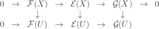
In this post, I would just like to discuss a slightly different perspective on the étale cohomology of varieties. This might be called the ‘relative’ or ‘monodromy’ perspective, and it is rife with geometric intuition. This perspective is certainly implicitly contained within all major texts on the topic, but is less emphasized as a good source of intuition.

NB: In this post I am sometimes lax with the distinction between and . In particular, one should assume that means everywhere.

Motivation

I discuss below two shortcomings with the perspective that “étale cohomology is the sheaf cohomology of abelian sheaves on the étale site”.

Virtues of a relative theory

Étale cohomology, or at least the parts shown in a first course, is often times introduced in a pretty absolute setting. This is the viewpoint, for example, that I took in this post. To every ‘space’ , we associate a vector space (or, more properly, a Galois representation) . We could then use this algebraic object to deduce things about or its relation to other .

What are examples of such things we can deduce? For example, this gives us a non-trivial means of classification— checking when . For example, as pointed out in this post one can deduce that and are not isomorphic by examining cohomology (technically, compactly supported cohomology, but same idea). The type of internal things one can tell about from are manifold. For example, if is a proper smooth variety over  a finite field , then ‘knows’ the size of for all . This is the content of Grothendieck’s trace formula.

There is one other good internal property that that is worth mentioning. If is a proper smooth variety over , a -adic field, then is good at picking up the reduction type of . In particular, if has a good reduction (meaning it admits a smooth proper model ), then (the inertia subgroup of ) acts trivially on . This follows from the smooth proper base change theorem. In fact, if is an abelian variety, then this is an if and only if statement (this is the Néron-Ogg-Shafarevich criterion).

So, all of these examples, and the many more I didn’t give, show why as an absolute, internal invariant of is an important object. But, much like most other cohomology theories one encounters, one gets a much more powerful, complete story if one thinks relatively instead of absolutely.

For example, if one is dealing with the normal (quasi)coherent cohomology of schemes, one has an absolute cohomology group for any (quasi)coherent : namely . This group tells you a lot about and/or in its absolute setting. Some obvious examples:

• One can deduce the genus of a curve (definitionally if over arbitrary , or less trivially over ) from the cohomology group .
• One can tell if the space is affine. Namely, the well-known criterion of Serre tells us that should be affine if and only if for all , and .
• One can tell if is projective. More specifically, one can tell if a line bundle is ample via Serre’s ampleness criterion.

But, by set-up, the groups are, themselves, not useful in discussing the relative properties of schemes. But, one can fix this.

This fix, of course, is furnished by the relative theory of the higher pushforward. Namely, given a map (with mild conditions, i.e. quasicompact and quasiseparated) one obtains a map which measures the ‘relative’ properties of the map . For example, is affine (ignoring some slight technical conditions) if and only if for all . Of course, we can recover the absolute, internal object by taking for a map which works because is a ‘trivial’ object, like a ‘point’ (and, of course, this works for any cohomologically trivial object–it works for any affine base scheme).

Similarly, in the topology of manifolds, one has the absolute notion of the singular cohomology , or, more generally for any sheaf of abelian groups (I’m being a little imprecise here, to know that ), one should assume that is locally contractible). I’m sure it goes without saying the important geometric content contained within . That said, just as in the last example, this absolute group tells you nothing about the relative theory of spaces. We need something more general to study the properties of maps . We’d like to know if is proper, or has connected fibers, or… ad infinitum.

This is given to us, similarly to the last example, by the relative theory of higher pushforwards. Namely, to a map we obtain a map . In good situations, such as if is proper (remember we’re working with manifolds!), or always, if we’re willing to work with ), the object is a sheaf on which ‘groups together’ the cohomology of the fibers (in the sense that its stalks are the cohomology of the fiber at that point). Thus, we will be able to capture the relative geometry of by studying its fibers which, once again with mild hypotheses, can be understood via these push-forward sheaves . Of course, once again, we can recover the absolute objects via if we consider maps to trivial objects: .

Thus, we’d like to have a similar relative theory in étale cohomology. Something that will allow us to understand the relative properties of maps, while, through this relative viewpoint, strengthening our view of the ‘absolute objects’.

Desire for fundamental group interaction

In topology one usually learns first about the fundamental group of a space . While I am not sure, it seems reasonable to me that ‘s preceding of (co)homology is mostly because it is much simpler intuitively. It’s easy to convince someone of the geometric importance/significance of studying loops on space up to contractions. One then studies the less intuitive objects , motivated usually the the statement that “we are trading in intuitiveness for computability”. And, indeed, the groups are much easier to compute, in practice, than the group (or more generally ).

Of course, the natural question one might ask is how these objects are related to one another. The first incarnation of the connection is via the identity: (assuming is path connected), which gives a very concrete measure of how is ‘simpler to compute’ than —we’re just eliminating all complicating non-commutativity. In the case of connected manifolds, this equality takes on a nicer form:

This equality is generalized by the, admittedly more complicated, Hurewicz’s theorem. Now, while Hurewicz’s theorem certainly provides a connection, it is much less satisfying in general than the case . It doesn’t make , or , seem any less ‘intuitive’.

Something similar happens in the theory of étale cohomology. One wants to study the ‘topological properties’ of a connected variety . The étale fundamental group is then introduced which gives a simple and easily motivated way of doing this. Namely, we study the ‘topological properties’ of by studying it’s ‘covers’, the maps which are ‘local isomorphisms’.

After the étale fundamental group, one then learns the definition of étale cohomology. After one’s been barraged with enough general theory of sites, and their associated topoi, one then mindlessly defines to be the right derived functor of the sections functor . One might be even more put-off once one sees the definition of compactly supported cohomology, or the actual definition of (the spiritual replacement for ).

Not only are these notions less ‘geometric’ feeling than one might hope (besides the obvious ‘they give the right answer is the right situations’, e.g. curves), they really seem far away from the more intuitive . Look hard enough and one will find statements like:

but these are often buried in texts. And this is usually the only real connection one usually makes between the ostensibly ungeometric and the more palatable .

A way of making things better

So, we shall try to remedy both of these issues. More specifically, we’ll begin by trying to strengthen our intuition for the relative theory of cohomology in the topological world. We’ll then adapt this to the case of étale cohomology, and reap all the rigorous and intuitive benefits that will follow accordingly.

The important notion in both cases will be the notion of monodromy. Something well-known to the geometers of the world, but which often times goes unmentioned in a first course on topology, let alone a first course on étale cohomology.

Monodromy in topology

Motivation

Monodromy is a pretty broad-use term (depending which part of the mathematical world you hail from), but is something that is probably well-known to anyone with an undergraduate degree in mathematics (at least secretly!). Very roughly, monodromy is the study of how an object changes as it passes around a ‘singularity’ of a space/map/whatever. The simplest incarnation of this is one of the first results one learns in an undergraduate course on complex analysis:

Theorem(Cauchy’s integral formula): Let be a holomorphic function on . Then,

Namely, we see that if we take the average value of as it travels around , that it picks up something interesting (translated: equals a non-zero number) if and only if it has a singularity at .

A much less effective, but more obviously topological, statement than Cauchy’s integral formula is what is sometimes called the ‘homotopy invariance of contour integrals’. Namely, if is a domain, and is holomorphic on , then homotopy equivalent loops in give the same contour integral. More rigorously, if (homotopic), for (for some chosen point ), then

One can recover the non-effective consequence of Cauchy’s integral formula (that having interesting average values around the circle iff it has a singularity at ) from this result: if is holomorphic on the disc, we can contract the loop to a point inside of the domain of definition of .

There is an even more fundamental incarnation of monodromy. One of the most basic differences between and is the lack of a good notion of logarithm. It is learned that one cannot define a holomorphic inverse to the exponential function . In fact, one often learns this through a sort of monodromy calculation. Namely, let’s suppose that there existed a complex logarithm on . Then,

but, by explicitly computing the left hand side (parameterizing the circle by ) one obtains that the left hand side is actually .

So, we calculated that as travels around the unit circle it picks up some interesting information which couldn’t happen if it had a global antiderivative—there is a monodromy theoretic obstruction to the existence of a global logarithm

Locally constant sheaves and the monodromy correspondence

So, we now begin in earnest in our rigorous discussion of monodromy. In this section, all of our will be path connected, locally path connected, and locally contractible. Nothing, in my view, is lost by assuming that is a connected manifold.

So, as one might expect, we define a sheaf of sets on to be locally constant if for all there exists a neighborhood of such that is constant. Note that, even though we just said that the restriction to a neighborhood of each point is constant, we didn’t actually say that they be isomorphic to the same constant sheaf. One might assume that we can have and . Of course, this cannot happen, else one can produce a disconnection of ! So, we will call the set such that the value set of .

Now, writing down examples of locally constant sheaves can be somewhat annoying, if one is not thinking about them in the right way. Namely, if one doesn’t realize that locally constant sheaves have something to do with topology, one might waste their time trying to write down locally constant sheaves on which are non-constant. We will see below that such a thing is impossible. But, in the interim, we offer the following example of a locally constant sheaf on the circle . Namely, consider the universal cover . One can then define to be the sheaf of sections of this map: (continuous maps). This is indeed locally constant since over any simply connected subset of , one sees that . The association being that is disjoint copies of (mapping homeomorphically to ) and so choosing a section is the same thing as choosing a copy. Clearly this association is actually an isomorphism of sheaves.

That said, the sheaf is not constant. Why? Well, for one thing it has no global sections. Any section of would need to be a homeomorphism onto its image, but doesn’t contain any copies of —a lowbrow reason for this is that all compacts connected subsets of look like closed intervals where removing two points needn’t disconnect it, but removing two points from always disconnects it.

This example was no accident. In fact, the locally constant sheaves on a space contain essentially the theory of covers of . Namely, we have the following theorem:

Theorem 1: The association to is an equivalence of categories:

The inverse map is given by the étalé space of . This should not be shocking. The general theory of the étalé space tells us that all sheaves of sets on are equal to the sheaf of sections of an étalé space over . Thus, the locally constant ones should correspond to étalé spaces which locally look like the étalé space associated to a constant sheaf . But, the étalé space of is the trivial cover

Thus, the étalé spaces associated to locally constant sheaves should thus be one which locally looks like the trivial cover or, in other words, a covering space!

Now, since locally free sheaves are the same thing as covers, and covers are informed/acted upon by (for a fixed, but arbitrary point ), we might expect there to be a non-trivial interaction between a locally free sheaf and the group . This action is precisely the notion of monodromy which will be important to us.

So, let us assume now that is a sheaf of -modules (not just sets), and we’ve fixed some . For any path based at , we can consider the pullback sheaf , which is a locally constant sheaf of -modules on . But, an elementary argument shows that any locally constant sheaf on is constant! Thus, we have canonical isomorphisms

Thus, by taking the inverse isomorphism of the first map, we obtain a canonical isomorphism . But, of course, there is also a canonical identification . Thus, since is a loop based at , we see that the above has produced a canonical isomorphism (of -modules!) . One might denote this automorphism . One can show, with a little work, that this definition only depends on the class of in , and thus we obtain a group map

called the monodromy action of on .

This seems totally reasonable technically, but what is visually going on? Let’s imagine that we have our locally constant sheaf of -modules on , and our fixed point sitting somewhere inside of it. Now, we can cover with a bunch of opens , corresponding to the neighborhoods where is constant. Let’s fix one that contains , call it Now, let’s think about our loop based at . As this loop makes its way around it will pass through several different . As it passes between such opens, we get an automorphism of the value group (which is non-canonically just !) from the transition maps between the neighborhoods. But, as makes full circle, it will land back where it started, in . The composition of these automorphisms then gives an automorphism of the value group on which is (now canonically!) . This is the monodromy action. So, to summarize the above picture in words—the monodromy action measures the change in the sheaf as it travels around the loop .

Phrasing the above a little differently (i.e. in terms of modules vs. representations) we see that the stalk has the structure of a (left) -module. In fact, one can show the following:

Theorem 2: The association is an equivalence of categories:

While this theorem is not terribly difficult to prove, the inverse functor is so nice, and so constructive, that it would a shame to not mention it. So, we want to go from an -module to a locally constant sheaf of -modules . The construction is made much simpler by considering the universal cover (which exists because of our hypotheses on ).

Namely, let’s begin by considering the constant sheaf of -modules on . We then define a sheaf on as follows:

A couple points should be made clear here. Namely, here we are thinking of the constant sheaf as being the sheaf associating to an open in the set of locally constant functions . Also, we are identifying with the group of deck transformations of . Thus, in the equality

the action of on the left is the action as deck transformations, and the element on the right is the action of on .

This definition may seem a little ad hoc, but is actually indicative of a general strategy in the theory of ‘locally constant things’. Namely, pull back our object to a cover where it must be trivial, and then provide ‘descent data’ about how to collapse/glue the trivial object back to our original object. So, in our case we have the universal cover . We know that for any locally constant sheaf on , the pullback will be constant (which is clear a posteriori from Theorem 2, or one can just show directly). But, is obtained from by ‘gluing dictated by —glibly,

Thus, something equally glib like should hold. But, that is precisely what we have described—sections of the quotient should be something like sections which transform correctly with respect to .

We should make one last remark on terminology. If, in the above, one lets be a field , and instead of all locally constant sheaves of -spaces, one instead focuses on the finite dimensional ones, then Theorem 2 easily reduces to the equivalence:

where has the obvious meaning. Now, locally constant sheaves of finite dimensional -spaces are often called -local systems. Then, also switching back to the representation theoretic viewpoint from before, we see that the above is also statable as an equivalence of categories:

where 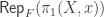denotes the category of finite dimensional representations (where will depend on —in fact, it’s just ).

Examples: locally constant sheaves on the circle

Let us now discuss the theory of locally constant sheaves on the circle . Why this example? Well, it’s non-trivial (it’s not simply connected) to be interesting, but trivial enough to be easily explained. Note that if we choose an orientation on , a distinguished loop , then we have the isomorphism with . From the last section we know that locally constant sheaves of abelian groups (i.e. -modules) on correspond to modules for the ring

But, of course, giving a -module is the same thing as giving an abelian group together with a fixed element (here this is automorphisms as abelian groups). Thus, we see that locally constant sheaves of abelian groups on correspond to abelian groups together with a fixed automorphism via the association

We will call the automorphism the monodromy operator for . Note that two such pairs and define the same locally constant sheaf if and only if there is a -equivariant isomorphism of groups.

This framework gives us a very convenient way of giving locally constant sheaves of abelian groups on . We will take full-advantage of this below in the discussion of examples on .

The first obvious example are pairs , where is an abelian group. As one might expect this uninteresting choice of monodromy operator (and is true in general!) corresponds exactly to the uninteresting type of locally constant sheaf—the constant ones. This is immediate from our construction of the sheaf associated to .

A non-trivial example might be the following. Consider the pair . In other words, the abelian group together with the automorphism corresponding to multiplication by . What is the locally constant sheaf that is associated to this? Well, we know literally what it is (we described them in general above), but let’s see more specifically what we get in this case. Namely, let be the associated locally constant abelian sheaf. Then, let us compute the sections  Here, .

We begin by noting that is going to be a subset of

Which ones? Well, it should be the such that

In other words, it’s just the constant functions picking out the elements such that . In other words, it’s just the constant functions picking out and . We will discuss the obvious generalization of this below.

Now, for the situation is slightly more complicated. Namely, our group will now be a subset of:

The last identification being the obvious one. In terms of locally constant functions, we’re looking for the ones such that

In terms of tuples, this translate to tuples such that

Thus, we really see that we’re getting the group . This should not be shocking. Since is contractible, we know that must be constant, and so must be .

The rest of the examples of locally constant sheaves of abelian groups on are equally as simple.

Cohomology and locally constant sheaves

In this section we will discuss two important issues involving cohomology and locally constant sheaves. The first will be how one can use cohomology to classify locally constant sheaves. The second will be concerned with the cohomology of the locally constant sheaves themselves. Both will be important in our translation of these facts to the setting of étale cohomology.

Classifying locally constant sheaves: the yoga of torsors

We begin by asking the obvious question: how many different locally constant sheaves on are there? How can they be classified? The key will follow from a very general fact concerning the notion of ‘twists’.

In an intentionally vague sense, a twist of an object is another object which is ‘locally isomorphic’ to . Twists show up everywhere in topology, algebraic geometry, etc.

As an example of a twist, besides the obvious (locally constant sheaves), think about the notion of a vector bundle in algebraic geometry and/or topology. Taking the former view, we’re looking for quasicoherent sheaves of -modules which are locally isomorphic to . In the latter, we’re looking for maps which are locally of the form . In both cases, we have a fixed object, namely (resp. ) and we’re looking for objects, namely quasicoherent sheaves (resp. maps to ) which locally on look like our objects.

Another good example are varieties which, over , look like some fixed variety —in other words, . Here the objects we are looking at are varieties, and the locality we’re trying to ‘trivialize’ (i.e. make isomorphic to on) on is the étale site of .

Now, the notion of twists is inextricably linked with a much scarier sounding term—I speak, of course, of torsors. For a sheaf of groups on a ‘space’ , a torsor is a sheaf of sets together with an action (of a group sheaf on a sheaf of sets) which is

1. Simply transitive—meaning that if is non-empty, then is a bijection for all .
2. has a ‘cover’ by ‘s such that .

My coyness in the usage of scare quotes should be obvious to some readers. Namely, the above makes sense on any generalization of a ‘space’, by which I mean a site.

Torsors sound exceedingly scary/abstract compared to the warm-and-fuzzy notion of twists. But, the two are not at all unrelated. In particular, associated to any twist of an object we have a naturally associated torsor. Namely, think of the sheaf which, as one might guess, associates to any the set of isomorphisms . This sheaf has the natural action of a sheaf of groups—the sheaf which, once again obviously, sends an open to the group (where should be taken to mean automorphisms preserving whatever structure and locally share). Indeed, an isomorphism composed with an automorphisms is another isomorphism. Moreover, this action is simply transitive. Finally, if and are twists, then there exists a cover by ‘s of such that , which gives that is non-empty. Thus, we see that is a -torsor.

Remark: Once again, I am being slightly imprecise here, beyond the obvious. To assume that the ‘isom sheaf’ is actually a sheaf, one should assume something more about the objects over the site with which we are working. Specifically, one should assume that they form a stack on the site.

One can then show that, in sufficiently nice situations (as in the one’s we will care about), there is a bijection between twists of and -torsors.

Now, in general there is a theorem that says that -torsors on a ‘space’ are classified by elements of . Note that one has to be careful in general as to how this cohomology ‘group’ is defined if is non-abelian. In fact, if is non-abelian, then it’s not really a group but a pointed set. If is abelian, then this is just usual sheaf cohomology.

Thus, putting this all together, we see that we get bijections:

As is clear, I am being intentionally vague here. One can make all of this precise. The first bijection is well-document, and can be found discussed here (they only discuss it for abelian sheaves, but it extends). The second arrow, inexplicably to me, is much less commonly discussed. The very rough idea is that the -cocycle form of elements of are precisely the ‘gluing instructions’ one needs to descend from ‘the pullback to a trivializing cover’—much like what happened with the universal cover and locally constant sheaves.

Also, if the automorphism group is abelian, then the cohomology group is an abelian group (vs. a pointed set), the torsors/twists have a natural group structure, and the bijection above is an isomorphism of groups.

This might seem a tad abstract, but you most likely have used this fact many times in your mathematical life. For example, the group of line bundles (i.e. twists of ) on a scheme is . By the above, we have an isomorphism

(where here is in the category of -modules), which is just the usual isomorphism!

We specialize all of this to our particular case to find:

Theorem 3: The set of locally constant sheaves of -modules on with value group is in bijection with .

Proof: Note that a locally constant sheaf with value group is the same thing as a sheaf of -modules which is a twist of the constant sheaf . Thus, by the above discussion of twists/torsors/cohomology we see that locally constant sheaves of -modules with value group should be classified by . Here the is with respect to the category of sheaves of -modules on . But, the equality

is clear, and so the theorem follows.

As a corollary, we are able to answer simple questions like: “how many locally constant sheaves with value group are there on ?” In particular, by the above, the answer to this question is

This was also obvious from the description of a locally constant sheaf of abelian groups with value group as a pair , with . The automorphisms of are just multiplication by and, one can show that these define inequivalent representations.  Thus, we again arrive at the number . This cohomological viewpoint is powerful in more difficult situations though.

Cohomology of locally constant sheaves

The other obvious question one could ask about locally constant sheaves is how their cohomology relates to their monodromy action.

As a sort of baby example, let’s think about the case of , where have a nice description of locally constant sheaves of -modules, as pairs . Let’s in particular fix a locally constant sheaf and have be its associated pair. Now, we want to compute the cohomology . Now, let be as above, and . Note that since and are contractible, that and are constant. But, since the cohomology of a constant sheaf is just the singular cohomology with values in the group (at least in the case of locally contractible spaces, which we are in), we can easily see that:

But, similarly, note that is the disjoint union of two contractible pieces, call them . Now, must be constant, and so using the same fact about the cohomology of a constant sheaf, we see that

Thus, by Leray’s theorem we may conclude that

So, in other words, we need to compute the cohomology of the complex:

which, obviously, as usual, sends

and

So, as per usual, we know that are the pairs whose image is zero, in other ones, those which agree on overlaps. So now, take such a pair . By the computation we did above, we see easily that

and

But, one finds when they attempt to compare these two, that the indexing is off by one (draw a picture, and it will be clear!). Thus, for these to agree on overlaps we actually need that . Thus, the elements are precisely the -fixed points of .

Using similar reasoning, if one thinks of as , the image of is going to be pairs . Thus, the cokernel of this map is .

This may seem somewhat inconsequential, and difficult to generalize, until one realizes that the above can be phrased as follows:

In other words, the first and second sheaf cohomology agrees with the first and second group cohomology of the monodromy action on the stalk! This turns out not be a coincidence, as we will now show.

Let’s begin with the easy part of this generalization:

Theorem 4: Let be a locally constant sheaf of -modules on . Then,

Proof: This is very easy by our description of the sheaf in terms of the monodromy action on . Namely,

But, since is connected, the are just the constant functions, and so we can easily identify this group with

To prove the corresponding statement for , we first need the following lemma:

Lemma 5: Let and be locally constant sheaves of -modules on . Then, for any short exact sequence of sheaves of -modules:

one has that is locally constant.

Proof: Since being locally constant is local we may as well assume that and are constant. Moreover, since is locally path connected, and locally conctractible, we may as well assume that is path connected and contractible. So now, let be any open connected set. Consider then the following ladder diagram

where the vertical maps are the restriction maps. Now, note that for exactness of the first row we are using the fact that is contractible. Indeed, this implies that if , for some abelian group , then . Thus, we do in fact have right exactness on the top row. A priori we don’t have right exactness on the bottom row since might not be simply connected.

Now, since and are constant, we know that the first and last vertical morphisms are isomorphisms. Thus, by the snake lemma we may conclude that the restriction map is an isomorphism. Thus, since is locally connected we may conclude that is just locally constant functions —i.e. it agrees, as abstract groups, with the constant sheaf.

So, let . Define the morphism in the obvious way. Namely, on any open with connected components define

One then easily sees that this defines the desired isomorphism.

Using, this we can deduce the hart part of the generalization of the situation for :

Theorem 6: Let be a locally constant sheaf of abelian groups on . Then,

where the cohomology on the right is group cohomology.

Proof: We note the following series of isomorphisms:

The content of the second equality was equivalent to that of Lemma 5 for the choice of (here is the category of locally constant abelian sheaves). The third equality follows from the equivalence of categories in Theorem 2, once again with . Finally, the last equality is by the definition of group cohomology.

Note that, in particular, for a constant sheaf we recover the well-known fact that:

since, of course, has trivial monodromy action.

Now, one might hope that we could extend the above to something of the form:

Of course, this is intuitively bound to fail. Namely, we already knew that was related to in some vague way. To think that is related to higher cohomology is just too much to hope for. As a concrete example, one sees that taking the above would imply that 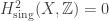if , which is, of course, ridiculous.

Remark: The spaces such that , for , all locally constant, and , are most likely well-known (at least by name) to the reader. Indeed, such a space is necessarily a —the Eilenberg-Maclane space for !

Higher pushforwards as transformations of local systems

We now discuss how one can think about the somewhat scary functors as doing something somewhat natural—of turning locally constant sheaves on the source, into locally constant sheaves on the target. Unfortunately, this isn’t universally true, and so we’ll need to remind ourselves a little bit of the situation we’re in (with regards to higher pushforwards) in the case of interest to us.

The inherent difficulty is that we’d like to say something like: “ is a locally constant sheaf of -modules if is”. Unfortunately, this does not hold in general. Before we give a concrete example, we recall a very, very powerful fact from sheaf theory:

Theorem 7(Proper Base Change): Let be a proper map, where is a manifold. Then, for any sheaf of abelian groups on , and any one has:

Recall that a continuous map is proper if it is closed and its fibers are all compact. Moreover, the sheaf on is just the sheaf , if is the inclusion map.

Remark: There is a much more general version of proper base changed, where one replaces with . In fact, using the analogous version of proper base change always holds. In reality, the version with is the ‘real’ version of proper base change. It’s just then a ‘coincidence’ that if is proper that .

We are also only mentioning proper base change in a very special case.  There is a natural generalization which says that if we have a fibered diagram of spaces

Then, we have a canonical isomorphism for any sheaf of abelian groups . Taking to be proper, and with the inclusion, recovers our version of proper base change.

For proofs of all of these things, one can read here.

With this theorem, we can easily create examples for which fails to take local systems to local systems.

As a first example, consider the space:

(here is the unit disc). We then have a natural map sending to . Visually, this is a family of elliptic curves over which degenerates to the cuspidal cubic at the origin.

We claim that is not locally constant, even though is. Indeed, if were locally constant, than since is contractible, we’d be able to conclude that is constant. Note though that by the proper base change theorem (since our map is indeed proper) we have:

To see this, note that for , we have that is the degree hypersurface in cut out by which, as one can check, is non-singular. Thus, is an elliptic curve (a non-singular cubic), and so topologically a torus.

That being said, is the plane curve , the cuspidal cubic. Topologically this is the two sphere . Indeed, consider the normalization map (thinking about this in terms of complex algebraic curves). As is easily calculated, , and moreover the map is bijective and proper (normalizations are finite for varieties!). But, this then implies that , being a proper continuous bijection must be a homeomorphism.

Thus, since has varying stalks, we may conclude that it is not locally constant (let alone constant!).

So, if we have any hope of having take local systems to local systems, we’ll need to consider a more restrictive class of morphisms than just topological maps. In fact, the above example even shows infinitely differentiable, proper maps between smooth (complex!) manifolds are not enough. One might sense, as was pointed out, that the lack of being a locally constant sheaf had something to do with the fact that was a degeneration. In other words, something about the singular fiber is messing with the preservation of being locally constant.

Thus, we should only be considering maps all of whose fibers are smooth. This turns out to be a bit of a red herring, as we’ll see below, but using this intuition we can guide ourselves to the right conditions. Namely, what makes a given  not smooth? It should be said here, as it can be confusing, that I am using smooth here in the sense of algebraic geometry (thus my choice of the phrase ‘infinitely differentiable’ before). So, a holomorphic map between, say, complex manifolds is smooth if it’s flat, and if its fibers are all non-singular. Now, the funny thing about smoothness, in algebraic geometry is that it does not correspond to smoothness(=infinitely differentiable)/holomorphicity in the smooth/holomorphic category. Indeed, what it best translates to is submersion. And, as one can check above, our is not a submersion.

It turns out that the addition of submersion is enough to imply something exceedingly strong:

Theorem 8(Ehresmann’s Theorem): Let and be smooth manifolds, and an infinitely differentiable, proper submersion. Then, is a locally trivial fibration.

Here being a locally trivial fibration means that there is an open cover of by ‘s such that is isomorphic (as spaces over ) to 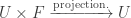for some space . A proof of Ehresmann’s theorem is just some good old differentiable topology. The proof can be found here, listed as Theorem 9.5.6.

One corollary of this is the following:

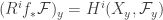
 Corollary 9: Let be an infinitely differentiable, proper submersion of smooth manifolds. Then, for any locally constant sheaf of -modules , the sheaf is locally constant.

Indeed, this is a condition which is local on , and so by Ehresmann’s theorem, we may assume that is just , from which it’s clear that is just the constant sheaf .

Remark: Note that since the cohomology of manifolds is finite dimensional, we can also see from this that sends local systems to local systems.

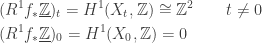
One can attempt compute some interesting examples of the above. It turns out, as is likely not shocking, that this is a difficult question in general. Let’s take, for example, the family of elliptic curves degenerating to a cuspidal cubic. As pointed out, is not locally constant. But, one can easily show that , where is a smooth proper map. Thus, is a locally constant sheaf on . But, is, topologically, . So, the same theory shows that is determined by its stalk at a point, and the action of the monodromy operator. By proper base change

as mentioned before. So, we just need to say what the monodromy operator is on this group to completely characterize the locally constant sheaf . It turns out that this operator is precisely . This is surprisingly hard to prove (its computation is contained within the Picard-Lefschetz formula), and contains deep information about the severity of the singularity at .

Thus, using all of the machinery we’ve developed we have the following nice interpretation of :

or, if we’re interested in local systems:

Thus, ‘relative cohomology’ (i.e. higher pushforwards) in this setting can be thought of as a means of translating the representation theory of to the representation theory of —to relate the covering theory of to the covering theory of .

This correspondence is not at all ‘easy’, indeed cohomology (while easier than homotopy) is still a difficult to understand object, but we at least know that it’s doing something fairly concrete. This, at least for me, is a clear-cut way of intuiting that their is ‘nice geometry’ in relative cohomology.

Monodromy in étale cohomology

We now seek to try and mimic what was done above, but in the case of étale cohomology. We’ll see, as was intended (or, so I would imagine) by the brilliant creators of the theory, that there is a rough one-to-one correspondence between what happened above, and what will happen below. We’ll see that we’re going to just have different words for different ideas, and some things (like locally constant sheaves) will be slightly more restricted objects, due mostly to the rigidity of the algebraic category.

Remark: In the below, I’m going to assume that the reader is familiar with the étale fundamental group. For those wanting to catch up on, or read more on this subject, I humbly believe that one can absolutely do no better than Szamuely’s book Galois Groups and Fundamental Groups.

Locally constant sheaves and the monodromy correspondence

We start, of course, with an adaptation of the notion of locally constant sheaves in the étale setting. Not shockingly, this is slightly more delicate than just the obvious definition: ‘a sheaf locally constant in the étale topology on ‘. The reason for this is something relatively intuitive. Whatever our definition of locally constant should mean, it should be both intuitive, but also do what we want it to do. In particular, we’d like some sort of equivalence between locally constants sheaves and covers (in the étale topology) and some non-trivial relationship to .

But, one of the brilliant insights that Grothendieck had was that even though étale maps, and more specifically the étale site , are the correct objects to capture the topological picture of , they are not exactly the right objects to capture the theory of its covers. Indeed, one should only consider finite étale covers. The reason being very simple: only the finite covering maps (in the topological world) will be algebraic. If we tried to include some sort of ‘infinite covers’ we’d end up with something which strictly leaves the world of schemes, and so becomes much more unruly to handle by algebraic methods.

Correspondingly, we shall essentially consider locally constant sheaves, but only those with finite value set. More specifically, we define a sheaf of sets on the étale site of (assumed, for the rest of this post, to be a geometrically connected, normal scheme) to be locally constant constructible (always abbreviated LCC) if there exists an étale cover such that is constant, with values in a finite set. By the same idea as in the case of spaces, the connectedness of forces them to have the same value set.

Remark: The phrase ‘locally constant constructible’ is a bit of an annoying one to a first time reader. Not shockingly, there exists the notion of a ‘constructible’ sheaf and, in fact, the LCC sheaves are precisely the locally constant constructible sheaves. Since we won’t be discussing the generality of constructible sheaves in this post, one should just take LCC as given, not part of some general theory. For our purposes, the phrase ‘locally constant finite’ would be more fitting, but that would buck too much against historical vocabulary, and be an inconvenience to a reader referencing other sources.

Now, the first thing one wants to check is that, as promised, this version of locally constant sheaf gives the correct analogue of the classical case, in so far as its relationship to covering spaces. The realization of this as follows:

Theorem 10: Let be a finite étale cover of . Then, the functor of points sheaf on is a LCC sheaf. Moreover, the association gives rise to an equivalence of categories:

I will not give a full-proof of the theorem here—one can be found, for example, in these notes of Conrad. The idea is roughly as follows. If is LCC then, by definition, it’s locally representable since the constant sheaf on is just , where is the disjoint union of copies of . But, the theory of descent tells us that things locally representable are representable. The fact that that the representing scheme is étale over can be checked étale locally (once again by descent), which is  trivially true. The fact that is a sheaf is, as usual, descent theory. The fact that it’s locally trivial follows an induction on the degree of .

But, there is another well-known category of objects equivalent to the category of finite étale covers of . Indeed, let us recall the definition of the fiber functor. We must first fix some geometric point (here is just some fixed separably closed field) of . We then have a functor which takes a finite étale cover to the set which is the ‘fiber’ of —the set of maps such that .

It follows from the ‘rigidity lemma for finite étale maps’ (that, at least for connected ones, they are determined by their value on geometric points) that is finite. Also, note that has an action of . Indeed, one can show that there is a canonical bijection between and for some sufficiently large pointed Galois cover . One then obtains an action of by its action on through the natural quotient map .

One can show that, in fact,

where the (co)limit ranges over a chosen compatible system of pointed Galois étale covers (running the gambit through the unpointed covers). This gives another interpretation of the action of which makes it seem less arbitrary.

This action, as we will see, is going to be the analogue of the monodromy action for LCC sheaves.

By construction (since it factors through a finite quotient) the action of on the finite set is continuous with given the discrete topology, and the profinite topology. In fact, one can easily show that this actually gives us a functor

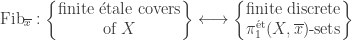
The following is not incredibly hard to show:

Theorem 11: The functor is an equivalence of categories.

Depending on how one first learned about , this may seem like an unmotivated way to think about covers—fiber functors sound very unappealing. That said, this is a purely geometric thing. If one defines the fiber functor in topology in the exact same way (except allowing for all covers and all discrete -sets) one obtains the same equivalence of categories. In fact, in both settings, if one so wished, they could define as being the automorphism group of the fiber functor.

Remark: These two cases of fiber functor/classifying group are not an isolated occurrence. In fact, if one so wished, they could develop the whole theory of ‘Galois categories’, and formulate this in a much broader context. This gives one a way of noticing ‘covering space/fundamental group like behavior’ in any situation. This is the point of view taken by Lenstra in his notes Galois Theory for Schemes.

Putting Theorems 10 and 11 together gives us a chain of equivalences:

with the associations being as follows:

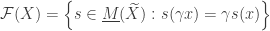
For our purposes, especially to make the analogy with monodromy more apparent, we’d like a way of describing the association of a finite discrete module to an LCC sheaf that doesn’t require going through finite étale covers. In fact, as one might hope, this association will be . The verification will be a simple unraveling of definitions, but due to the importance of the result for us, we discuss it below.

We begin by recalling the definition of :

as travels over the pointed étale maps . In other words, is where is our geometric point. But, note then that since is locally constant we take some finite Galois étale cover such that is constant (the fact that we can take finite follows from the finiteness condition of being LCC, and the fact that we can take Galois is just the fact that all finite étale covers are covered by a finite Galois one).

Thus, we can clearly identify with .  But, this has an action of through, as before, the quotient map . But, note that if , then this is precisely the finite discrete -set we associated to . Thus, the fiber, with the action described above, really is the result of Thus the correspondence between LCC and finite -sets is .

So, now, restricting our selves to abelian LCC sheaves (i.e. LCC sheaves of abelian groups), we easily deduce from the above an equivalence of categories:

Theorem 12: The association is an equivalence of categories:

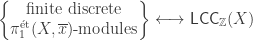
Where, of course, denotes the category of abelian LCC sheaves. In fact, with literally no extra work one can sup this up to an equivalence of categories:

This is precisely the analogy of the monodromy correspondence that we might have wanted. And, as expected, it follows very similarly (through formal manipulation) from the definitions of the fundamental group and ‘locally constant’ sheaves.

We’d like to make one final important remark in this section. In Theorem 12 above we basically took the ‘abelian part’ of the correspondence between finite discrete -sets and LCC sheaves. But, to have a full picture of the ‘abelianized’ situation, we’d like to have an analogy to Theorem 10. Namely, what happens to the middle category in the set-theoretic world of LCC things? Namely, what type of finite étale covers do abelian LCC sheaves correspond to?

The answer is both unsurprising and extremely powerful. Namely, let us recall that a finite commutative étale group scheme is a commutative group scheme whose structure morphism is both finite and étale. One can easily then trace through the above to fill in the missing link for the ‘abelianized’ version of the set-theoretic situation. Namely, we have equivalences of categories:

Some examples

We now pause to give some examples of the above theory. By the very last set of equivalences in the previous section, we have multiple ways to present an abelian LCC sheaf to the reader, and we explore these different presentations.

• As a first, and most trivial example, we can consider the ‘constant’ objects. For example, we could consider the abelian LCC sheaf where is just any finite abelian group. This corresponds to the finite commutative étale group scheme given as a scheme by

  

  and with multiplication map:

  

  as just the map which sends the -copy of to the copy, and with the obvious identity section/inverse map. The finite -module associated to is just the abelian group with trivial action. Thus, we see that this is entirely analogous to the case of constant sheaves in the topological setting.

• As a much less trivial example, we can consider a -variety , and the object on , where satisfies . As a sheaf we can define as follows:

  

  with the obvious group structure. To see that this is actually finite étale, one can proceed as follows. Since , the extension is finite separable (here is a primitive -root). Thus, the map from the obvious base change is finite étale. One can then check that is just the constant sheaf . Thus, is an abelian LCC sheaf.

  As a finite commutative étale group scheme, is just (here is relative spec) with the obvious addition, inversion, and identity section. One can alternatively define over as , and then over is just the group scheme one obtains as .

  Lastly, we can describe as a finite -module as follows. Note that since becomes constant, equal to (the second isomorphism is non-canonical) over we see that our of on  comes through the factorizations

  

  And, the action of on is the usual one.

• As a last example, let’s consider some field. Consider then an elliptic curve (or, more generally, an abelian variety). Then, for we have a finite étale commutative group scheme given by , where is the multiplication by map. It is a classical fact to show that is, as claimed, étale and, in fact, .The description of as an étale sheaf is simple, but not very enlightening (considering we haven’t said anything substantive about ). Namely, let be an étale map. Then, as is well-known, is a disjoint union of covers where is a finite separable extension. So, to say what is, we need only say what is, and then take the corresponding product. Now, is just, definitionally, . This is not too helpful intuition wise though. If one thinks of as identified with (as is done in ‘classical’ algebraic geometry), then are just the torsion points of the group with coordinates lying in .
  
  Finally, we need to describe as a module over (here means separable closure). Once again, this is most concretely thought about in the classical view of . Namely, think of as . Consider then , where means adjoin to all coordinates of all the tuples in (note that we said there are finitely many of them— to be exact). It’s then clear from the discussion above that is finite Galois and, in fact, (as a sheaf) becomes trivial over . With this view, the -module associated to is the group acted on by through the quotient which acts on the pairs in diagonally.

Now, as in the last example, we see that over , LCC sheaves just correspond to finite -modules. Indeed, this is just the equivalence of Theorem 12. We are particularly adept, as students of arithmetic, at asking questions about Galois modules/representations. In particular, an interesting question is when, for a -adic local field, the Galois representation associated to an LCC sheaf/finite commutative étale group scheme is unramified. The following gives a very satisfying answer:

Theorem 13: Let be a -adic local field. Then, a finite commutative étale group scheme has unramified associated Galois representation if and only if extends to a finite commutative étale group scheme .

Proof: Suppose first that extends to some over . Now, it’s plain to see that the module associated with is with the obvious action. Similarly, the module associated with is with the obvious action. Now, note that we have a natural map

which is actually -equivariant. Of course, even though the monodromy action on is an action of it still has a -action. But, note that we also have a natural reduction map

where here is the residue field of . This map clearly intertwines the natural map .

The important observation though is that both of these maps are isomorphisms. Indeed, , , and . But, note that since each of are étale, we must have that each of , and are constant with the same value group. Since the maps we described are just the identity maps, the conclusion follows.

The unramifiedness comes from the fact that acts trivially on which is -equivariantly isomorphic to .

Suppose now that is unramified. This means that the action of must factor through some finite Galois group with unramified. But, one can then see that this implies that becomes constant (as a group scheme) over .

So, for simplicity, let’s assume that is integral. One can adapt the proof with some work to the non-integral case. Then, we can consider the normalization of in —call it . Note that still has group operations. Indeed, if , we want to define group operations on the integral closure of in . But, since is integral, the Hopf algebra operations obviously extend to , and then one can see that since they are finite, they restrict to map between the integral closure of . So, we have a group scheme which is a lift of , but it’s not obvious it’s étale. But, the key is that must be the normalization of in the constant group scheme , which is constant. Since is étale, the conclusion follows.

Remark: One could kill the first part of this theorem, as one kills a fly with a Howitzer, with smooth proper base change.

To end this section, we’d like to give sone non-examples of finite commutative étale group schemes (and/or LCC sheaves and/or finite discrete -modules).

• Consider , defined in the exact same fashion, over . This is an example of a finite commutative group scheme which is not étale. Indeed, note that since has characteristic , one has that for all finite separable extensions . Thus, if it were étale, then by our correspondence, it would need to correspond to the trivial group scheme, but it does not. More directly, it’s easy to see that the structure map is not étale. If it were, then would need to be reduced, but it’s not.
• Let be an elliptic curve. Then, is a commutative finite group scheme over but never étale. Indeed, suppose that were étale. Then, the map would have étale fiber over . But, since this is a map of group schemes, this would imply that is actually étale. But, it’s well-known that it’s not. In fact, it’s not even separable since the induced map to itself (here is the generic point) is the zero map—it’s just multiplication by , which is zero.
  
  An alternative way to see the non-étaleness is as follows. Note that we have the natural relative Frobenius map (you can look here for a reminder on its basic facts) is a group map since it preserves the identity. But, since , we know that is a finite flat commutative group scheme over of degree . Thus, (this is reasonably easy, albeit tedious, result of Deligne—see page 19 of these set of notes ) and so . But, clearly is the one point set. But, this implies that can’t have points. But, if were étale, this would need to be the case.

Cohomology and LCC sheaves

Now, just as before, we’re going to give a cohomological study of LCC sheaves. And, again just as before, this will be broken in to two pieces. First the study of twists of sheaves which will allow us to try and classify LCC sheaves on a scheme. Second, a study of the cohomology of LCC sheaves themselves.

Classifying locally constant sheaves: the yoga of torsors

Just as before, the content of this section will be the bijection

But, now everything should be considered in the étale topology. So, a more accurate correspondence would be

Here are some examples to wet our whistle before we jump straight into the case of LCC sheaves.

• Let’s suppose that we wanted to classify twists of on . In other words, we want to classify schemes such that for some finite separable extension . Equivalently, we want to classify such that (here, again, means separable closure). Such objects are called Brauer-Séveri varieties of dimension . The above tells us that such things should be classified by . But, as is always the case, one can identify étale cohomology with Galois cohomology by taking fibers. In particular, we have:

  

  where we have used that the stalk at a geometric point of the sheaf is (note that one should be careful—one of these ‘s is sheaf Aut [as in the case of classifying twists] and the other is just the automorphism group). The action of on , as one can easily check, is the expected one.

• As another example, let’s suppose that we wanted to classify central simple algebras (of degree ) over . You’ll recall that one definition of such objects is algebras such that for some finite separable extension . In other words, they are algebras such that . The theory of twists then tells us that we can classify central simple algebras by (thinking here, as usual, of as being a sheaf of algebras on ). Applying the étale-Galois comparison theorem again, we see that twists should be classified by . But, as is well-known (it’s a very baby case of the Skolem-Noether theorem) one has that . Thus, central simple algebras of degree Are classified by .
  
  Thus, we see that there is a correspondence between dimension Brauer-Séveri varieties over , and degree central simple algebras! The correspondence is fairly explicit. For example, if one takes the quaternion algebra , this is associated to the Brauer-Séveri variety . This is smooth, and so (using the genus-degree formula) genus . Since geometrically (i.e. over ) all genus zero curves are , we may conclude that is indeed a Brauer-Séveri variety of dimension . If one would like to learn more about these objects and their correspondence I can give no higher recommendation than to Szamuely’s book Galois Cohomology and Central Simple Algebras.

  Remark: Of course, the set of central simple algebras on is the Brauer group of . There is a natural group operation on the set (see Szamuely’s book) which natural then identifies it with . A common identification one wants to make over a field is . This is very naturally described thinking in terms of twists as being the result of taking the direct limit of the maps

  

  one obtains from the long exact sequence coming from the short exact sequence

  

  The injectivity of this map follows, essentially, from Hilbert’s theorem 90, by examining the previous term in the long exact sequence. The surjectivity is hard, and can fail in more general algebro-geometric objects. For more discussion of this, and of Brauer groups in general, see this post.

• As another example, one can try and classify ‘étale line bundles’. In other words, quasicoherent sheaves of -modules on locally isomorphic to (one needn’t, of course, assume that the sheaf is quasicoherent—that follows for free). The theory of twists tells us that such a thing is classified by . But, of course, . So, we see that étale line bundles are classified by . But, it’s not hard to show that all étale line bundles are just the ‘étalification’ of Zariski line bundles. This follows from the more general equivalence of categories of quasicoherent modules and those on . In particular, we may conclude that . This is an example where the theory of twists is helpful in determining a cohomology group, not the other way around.

So, let us now turn our attention to classifying locally constant sheaves using this theory of twists. To begin, note that a sheaf locally (in the étale topology) isomorphic to a finite abelian group is automatically LCC, and in fact, these are clearly exactly the LCC sheaves. Thus, classifying LCC sheaves which are locally isomorphic to the constant sheaf is the same thing as classifying all abelian sheaves which are locally isomorphic to .

So, the theory of twists/torsors tells us that we have a bijection

But, as is patently clear, we have a canonical identification of with (here is as abelian groups). Thus, the sheaves on étale locally isomorphic to are in bijection with .

Now, while this may sound like a pretty contentless result, a little thought shows that it really is not. Indeed, unlike singular cohomology which is relatively simple to compute, étale cohomology is decidedly harder. Take for example something extremely simple like . What is this? If this is well-known, it’s . But, what if ?  Even if one sticks to the computation of even simple groups like can be quite hard and is, as you well-know, the main content of the computation of the group .

But, even though the level of difficulty in computation has jumped significantly from the situation in topology, this result is still extremely useful. For one, it gives one a reasonable means to compute twists/locally constant sheaves. Without the above equivalence, trying to decide how many non-isomorphic local systems there are on seems like a completely unapproachable problem. This equivalence allows us to appeal to the manifold tools that exist in the theory of cohomology. One of the most important being the relationship between the cohomology of different sheaves.

Lastly, we can, from various abstract theorems about cohomology, immediately deduce some bare-bones finiteness results. For example, if is a sufficiently nice variety (e.g. smooth projective) then the finiteness theorems from étale cohomology tell us that there are only finitely many twists of for any, say, finite cyclic group of order coprime to .

All of this philosophizing aside, we should use the above equivalence to at least compute the size of the set of twists of some simple groups on some simple spaces.

Let us show that if (here is a power of the prime ) is a variety (still under the blanket assumption of geometrically connected), then the number of LCC sheaves locally isomorphic to is practically computable, and is finite in reasonable situations (e.g. proper). The key will be the so-called Artin-Schreier sequence. Indeed, consider the following short exact sequence of sheaves on the étale site:

It is defined by the first map being the inclusion, and the second map being (on points) . One can check that this is indeed a short exact sequence of abelian sheaves. Thus, we get the following exact sequence as a portion of the long exact sequence

But, note that . Thus, as is well-known, we can replace with (coherent cohomology on the Zariski site!). Thus, we see that we can compute entirely in terms of coherent cohomology which is practically simple. As an example, one can easily compute that as expected.

Cohomology of locally constant sheaves

We now turn to the question of how to compute the cohomology of an abelian LCC sheaf on . In a perfect world, one would hope that we’ll encounter a situation very similar to the topological one. In fact, we will, and, amazingly, roughly the same method of reasoning will show this.

Let us begin by noting that, just as before, the subcategory of abelian LCC sheaves is closed under extensions in the larger subcategory (it’s a so-called ‘weak Serre subcategory’). Said more precisely:

Lemma 14: Suppose that sits in a short exact sequence

where and are abelian LCC sheaves. Then, is an abelian LCC sheaf.

Proof: The proof is not very hard. One just essentially reduces to the constant case and writes down the generators for . A full proof can be found here.

With this, we can proceed just as in the topological case to show that the first cohomology of locally constant sheaves can be computed just using the monodromy action:

Theorem 15: Let be an abelian LCC sheaf on . Then, we have the following isomorphism:

where the right hand side is continuous group cohomology.

While the line of reasoning will be very similar to the proof of Theorem 6, there is one very clear-cut difference. Namely, we no longer can use —it’s not an LCC sheaf. Thus, we will have to be a little more clever with our manipulations.

Proof: Let have value group of order . Note then that is actually an element of (the category of locally constant sheaves of -modules). We begin by noting that using the standard arguments (cf. Prop. 2.6 of Hartshorne) that computing is the same thing as computing the cohomology in the category of sheaves of -modules on —in other words,

which is well-known (loc. cit.).

But, note then that the cohomology of in is just . Now, Lemma 14 shows that this is the same as . But, by the equivalence of categories discussed immediately after Theorem 12, this is the same thing as where is the category of discrete -modules (note that we can work in the full category of modules since any extension will necessarily be finite). But, this is evidently equal to , where is the category of discrete -modules. But, this is equal to the continuous group cohomology, as desired.

Of course, as a corollary, we obtain the well-known easy case:

Corollary 16: Let be a finite abelian group. Then,

This just follows from the fact that the first continuous cohomology of a trivial module is the group of continuous homomorphisms to that module.

Applications of Theorem 15

Somewhat differently than in the topological setting, it often times happens that it’s easier to get one’s hands on than (the étale cohomology analogue of singular cohomology with coefficients). The reason for this is twofold.

First, the ease of computation of in the topological context often times comes from the nice existence of Leray covers for , or the existence of nice cellular decompositions of . For étale cohomology it’s difficult to find Leray covers, and there is no analogue of cellular decomposition. Second, the connection to the geometry of is much clearer for than it is for . This often times allows one to get extra leverage on the computation of inaccessible to .

But, the above theorem allows us to get a fairly complete handle on using . We discuss below some of the benefits that can be reaped from this connection:

Cohomology of affine space

We claim that for any of characteristic ( may be ) that for and . By the Kunneth formula, it suffices to verify this for . Moreover, by standard dimension theory for étale cohomology for . For , we know by Poincaré duality that this is equal to which trivially equals zero. Thus, we’re only left to compute .

To show this is zero, we need only show that for all . But, by Corollary 16 this is equal to . We claim that this is zero.

We need to be slightly careful with this though. Recall that the equality holds only for characteristic zero. Indeed, for characteristic a theorem of Raynaud (cf. Theorem 4.9.5 of Szamuely’s Galois Groups and Fundamental Groups) says that is ungodly large. But, the key is the following: all finite continuous quotients of have no prime -quotients.

To see this, suppose that has a prime to finite continuous quotient . Then, by the standard theory we know that there exists some finite connected étale Galois cover with . Now, since is smooth and integral over , we know that is smooth and integral. Thus, we can choose a projective model for it. Let be the map obtained by the curve-to-projective theorem (i.e. the valuative criterion for properness). This is a finite Galois cover.

Note that the degree of the map is . We claim that this implies that is tamely ramified. Indeed, since the map is Galois if we have that (where is the ramification index at any point ). Clearly then since . Note then that by standard curve theory, the degree of the ramification divisor of at is . Thus, from Hurwitz theorem we obtain

But,

Thus, this forces . A moment’s thought then forces , which is a contradiction.

Cohomology over integer rings

Let be a finite commutative étale group scheme over , where is a number field, and is a finite set of primes, and let . Note then that (where is the obvious geometric point ) is , where is the algebraic maximal extension of unramified outside of . Moreover, as a -module is just with the obvious -action. Theorem 15 then shows that

In particular, note that if one takes and the above says that

Indeed, ! This says that étale cohomology over , at least the cohomology of LCC sheaves, is silly.

Another nice application of this is the following. In the proof of the weak Mordell-Weil theorem, the critical part of the argument is that if has good reduction away from , then where , and show this latter group is finite. To see how one obtains such an injection, consider that since has good reduction away from one has an abelian variety , where (we could have taken one over !). But, also note that the sequence

is exact, where the second map is multiplication by . Taking the long exact sequence in étale cohomology gives

In particular, we see that we get an injection . But, by the valuative criterion, , and by the above we have the equality

This is how we obtain the desired injection.

Remark: This also naturally comes up in an analysis of Mazur’s torsion paper. Namely, there is a key step where he needs to make the switch from Galois(=étale) cohomology to fppf cohomology. The main reason for this need to switch is illustrated above since the étale cohomology over , which is what one may be led to believe is the correct choice, is not very rich. For more information, see here.

Higher pushforwards as transformations of local systems

Finally, we come to how higher pushforwards fit into this monodromy-focused way of thinking, and how it can help sharpen and consolidate our understanding of various parts of the definition of étale cohomology.

So, just as before, the goal is to say something like “the (higher) pushforwards of LCC sheaves are LCC”. And, just as before, this fails even in fairly tame situations. In fact, let’s consider the exact analogue of the counter-example we did in the topological setting. Namely, let’s consider

with the obvious mapping . We note that satisfies similarly nice properties to its topological analogue. In particular, it’s a morphism, the analogue of holomorphic and it’s proper, the analogue of topologically proper. That said, we claim that is not LCC. We basically leverage the same proof as before using the étale analogue of proper base change:

Theorem 17(Proper base change): Let be a proper morphism of schemes. Then, for any fibered diagram as follows:

and for any torsion abelian sheaf on the canonical morphism

is an isomorphism.

Proof: The proof is considerably, considerably harder than the topological analogue. Anyone wanting to spend a few hours of their life (at a minimum), and who loves dévissage to can look here.

Anyways, appealing to this, we may conclude (in our very baby case) that cannot be LCC. Indeed, let be the obvious geometric point then

since is an elliptic curve.

But, if is the obvious geometric point then

since is the cuspidal cubic. This computation can be done one of two ways. Using smooth-proper base change, one can reduce to the case of , which we’ve already done. Alternatively, using the ideas in this post one has a short exact sequence of sheaves on given by

where is the obvious inclusion, and likewise (here is two points). We then get a long exact sequence, a portion of which reads (after simplifying obvious terms)

Replacing the first two obvious terms, and noting that is just which we’ve already computed to be we get the sequence

from where the conclusion follows.

Regardless, we see from these computations that cannot be LCC.

We may then think that the next natural step is to say “but by some analogue of Ehresmann’s theorem if is smooth proper then we’re OK” and then finish our discussion. While this is a reasonable thing to do, we’ll get a lot more milage by first trying to move from the land of finite coefficients to the land of non-torsion coefficients. Of course, as remarked in the section on LCC sheaves, one cannot literally hope to do this by using some notion of ‘locally constant sheaf’, but as was Grothendieck’s brilliant insight, things are made OK by viewing these non-torsion sheaves as being formal projective systems of torsion sheaves.

The category of lisse sheaves

Basic definitions

As was alluded to at the end of the last section, our goal is to pass from the category of LCC sheaves to something more understandable—categories of non-torsion ‘locally constant sheaves’. The ideas in this section, while highly non-obvious and ground breaking ideas of Grothendieck, are something the learned reader may already be well-acquainted with. The insight is closely related to the deceiving nature of denoting the -adic cohomology of a variety by . The deception comes from the fact that we’re not really taking cohomology of a sheaf with values in . Indeed, the actual definition of -adic cohomology is

The idea is that while only the sheaves make sense as ‘algebraic objects’ (e.g. correspond to algebraic covers) the inverse limit above acts like it’s really the cohomology of the constant sheaf .

Remark: The recent work of Bhatt and Scholze show that if one is willing to eschew the comfortable étale for the pro-étale one can actually make sense of -adic cohomology as the cohomology of a constant sheaf (of topological rings).

The idea now is to generalize/imitate this idea by trying to create a category of ‘locally constant’ -sheaves. Now, one test of the usefulness of such a theory will be the existence of theorems for these sheaves analogous to those we had for LCC sheaves. In particular, we’re going to want an equivalence of categories between ‘locally constant -sheaves’ and the category continuous representations .

So, let us begin by defining precisely what we mean by the category of ‘projective systems of locally constant sheaves’. We shall call this category the category of lisse (this is the French word for ‘smooth’) -sheaves on (or if we want to be extra careful). We shall denote this category by . For notational ease, let us denote the constant sheaf of rings on with values in by .

Not shockingly the objects of are projective systems satisfying

where in the map is the one coming from the specified map and where is a -module via the usual reduction map. A morphism in from to is just a morphism of projective systems, where is -linear. We shall denote the set of morphisms from to by . It’s a group, that much is clear. But, a little thought shows that it’s also a -module.

Let us now give the two most important examples of lisse -sheaves on :

• Let us take with the usual reduction maps . This system clearly satisfies the conditions to be a lisse -sheaf on . We shall denote it (no confusion should arise).
• Let us assume that is invertible on . Then, let us consider the projective system with the map being the -power map. It’s clear that this is also a lisse -sheaf on —although note that it was important that is invertible on , so that each is LCC. We shall denote this lisse -sheaf by . It is often called the ‘Tate twist’.
• For any LCC sheaf of -modules , one can create a lisse sheaf also denoted . Indeed, define for , and for , with the obvious system of maps. This gives a fully-faithful embedding of the category of all “-torsion LCC sheaves” into the category of lisse sheaves.

The idea behind lisse -sheaves is the following. We think of each system as being something of an ‘avatar’ for its inverse image sheaf which, since each is LCC should be ‘locally constant’. But, as set-up the sheaf would be a sheaf of modules over . Thus, lisse -sheaves is our replacement for the category of ‘locally constant sheaves of -modules’ on .

Now, as one would hope, the category is abelian. Things go through mostly as expected, with one slight hiccup. To understand the root cause of this complication, we consider the following example. Since the lisse -sheaf is our avatar for the constant sheaf we’d better believe that it acts similarly. In particular, if we consider the natural ‘multiplication by ‘ map given by for all , then we’d hope that this would be injective.

Of course, we see an issue. If we try to do something naive like define to be the lisse -sheaf with , then the kernel of would be non-trivial. The problem is that even though we’re shackled to the world of projective systems (because of the complication of non-torsion sheaves), we should always be thinking about their associated avatars—their inverse limit. In particular, we’re looking to capture the kernel in the category of ‘inverse limit sheaves’.

This is achieved as follows:

where the map is the one coming the map . This says precisely that the elements in the -entry of should be those coming from something living in all the kernels of above it. This is precisely what should happen in the category of ‘inverse limit sheaves’. One can then check that with this definition is indeed injective.

So, with this correct definition of kernel and the more naive definition of cokernel (thinking about inverse limits should tell you why the naive definition here is OK) one can prove that is indeed abelian. Of course, one should show that these operations don’t actually leave our category (fleeing into the larger category of projective systems of abelian sheaves)—in other words, one should verify that these are actually projective systems of LCC sheaves. This is not difficult, and should be checked only by the skeptical.

One can also easily check that also enjoys the usual cadre of operations. In particular, one can take the tensor product of two lisse -sheaves (defined coordinate-by-coordinate) is a a lisse -sheaf. Similarly, one can show that for any two lisse -sheaves and the ‘sheaf hom’

with the obvious structure is an element of .

Now, lastly, we want to define a lisse -sheaf, whose category will be denoted . This is another object which, at first glance, seems somewhat unnatural. But, as per usual, the key is to try and keep its ‘avatar’ in mind. What we want to imagine is that if is lisse -sheaf, with avatar (remember, this is just for intuition!) then we can tensor this locally constant sheaf of -modules with to obtain a locally constant sheaf of -modules. Of course, the operation of literally tensoring a system with is unavailable to us.

The workaround to this issue is something fairly common, but can be jarring if it’s one’s first exposure. To motivate it, recall that if is a field then one has two important categories involving abelian varieties over . On one hand, we have just the usual category of abelian varieties . But, we also have the important category which is supposed to act like a category of ‘isogeny classes of abelian varieties over ‘.

That said, does not have such things as its objects. In fact, the underlying object class of is the same as —what differs is the class of morphisms. Indeed, is abelian category in an obvious way, and so is an abelian group. One then defines

the idea being that and are isogenous if and only if they are isomorphic in . Thus, while is not really a category of isogeny classes of abelian varieties, it acts in very much the same way (it’s ‘skeletonized’ by such a category).

A similar idea will work for us. We want to imagine that the objects of the category are classes of sheaves—a class consisting of sheaves which become equal when one ‘tensors with . But, as we’ve said, the tensoring operation is problematic, and so we take a cue from the previous paragraph. Namely, the objects of will be the same as the objects of , but we define the morphism group as follows:

For notational convenience, we shall denote by . Also, when we want to emphasize that we’re thinking of in versus , we might denote it by (even though, really, it’s the same object).

As an example, let’s consider the lisse sheaf (as described in the third example of lisse -sheaves above). Clearly we want this object to be when thought of as an element of . To see that this does in fact hold true, one needs merely check that , but this is clear by inspection. Thus, .

Remark: If one wants to work harder, they can create the category of lisse -sheaves. Indeed, one first defines the category of lisse -sheaves, for all finite—it’s just the category of projective systems of -modules (where is a uniformizer) with the obvious properties. One then defines the category of lisse sheaves in a way completely analogous to the construction of lisse -sheaves. Finally, one defines the category of lisse -sheaves to be the direct limit of the categories over all finite extensions . This seems entirely formal and obvious (given the above construction), except one small point. Why are we forcing lisse -sheaves to live as a lisse -sheaf for some finite —why not allow ‘infinite degree’ analogues? This is a good question, and will be answered in the next section.

Monodromy correspondence and cohomological properties

As mentioned before, the above definition of a ‘locally constant -sheaf’ will only be worth its salt if it acts in expected ways. In particular, we’d hope, looking back to the topological/LCC setting, that lisse sheaves have a notion of monodromy. We’d also hope that we can understand their first cohomology groups using this monodromy action. Both of these will holds true, and are largely just formal consequences of the analogous results for LCC sheaves. That said, they are important enough that we restate them here.

Let us begin by defining what we mean by the stalk of a lisse -sheaf on at a geometric point of . Begin by noting that if is a lisse -sheaves, then the morphisms give rise to maps of abelian groups . We thus obtain a projective system of abelian groups .

Moreover, note that using the defining properties of a lisse -sheaf we have that each is a -module, and that the map intertwines the module structure with respect to the usual ring map . Thus, we see that the inverse limit is naturally a -module. This is what we call the stalk of at the geometric point .

Remark: Note that we can actually realize the ‘avatar’ of in terms of its stalks—thanks mainly to the fact that while LCC sheaves do not have nice inverse limits, modules do!

Note, moreover, that has more than just the structure of a -module. Namely, we know from the LCC theory that each naturally has the structure of a discrete -module. Moreover, the map is a map of -modules. Thus, we see that inherits the structure of a continuous -module. But, acts -linearly (by construction) and so what we really obtain is a continuous homomorphism called the monodromy representation associated to . Another way of phrasing this, is that is a continuous -module (the continuity just meaning that acts continuously).

As one might hope, we have the following:

Theorem 18: The association is an equivalence of categories:

The proof of this proposition follows from formal manipulations of Theorem 12.

While this version is nice, it’s the version for lisse -sheaves that is perhaps even more striking. Let us begin by defining, for a lisse -sheaf the stalk at a geometric point . Not shockingly, it will just be the continuous -module one obtains from tensoring with . Thus, not shockingly we shall denote it . Since all finitely generated -modules are free, Theorem 18 becomes the following very important theorem:

Theorem 19: There is an equivalence of categories

The category on the right hand side denotes the category of finite dimensional continuous representations of for various .

This is great, but to make the analogy between lisse sheaves and usual torsion free locally constant sheaves complete, we want to verify that something like Theorem 6 holds. But, this is a purely formal consequence of the definitions. Indeed, before we can even begin to ask if such a theorem can hold for lisse sheaves, we need to define what the cohomology of a lisse sheaf means. In particular, let’s suppose that is a lisse -sheaf on . We then define the cohomology of it as follows:

where the projective system on the right hand side is the one coming from the projective system after applying the functoriality (in the sheaf entry) of cohomology.

Since each is a -sheaf, the cohomology is a -module. And, of course, using the defining characteristics of a lisse -sheaves, the aforementioned projective system intertwines the module structures. Thus, is naturally a -module. This then allows us to define the cohomology of a lisse -sheaf:

as one would expect.

This, honestly, seems like a bit of a cop out. Sure, this is the analogy of the usual definition of -adic cohomology, but why is that defined as it is? One of our goals of developing this relative theory was to clarify and demystify the definition of -adic cohomology, and tease out some of its more geometric figures. We have seemingly done nothing but furthered the formalism, without adding any intuition. Don’t worry though dear friend. In the next section we will (try to) make clear the intuition behind this definition. But, for now, let us just take it as given.

So, with this definition, the analogue of Theorem 6 follows almost immediately:

Theorem 20: Let be a lisse -sheaf (or -sheaf) on . Then,

where, as before, the right hand side is continuous group cohomology.

Proof: We prove the case when is a -sheaf, as the -sheaf case is then just a formal consequence. Note though that we have the following:

as desired.

The étale relative theory

We are now prepared to take this monodromy theoretic approach to the relative setting. As one would expect, we shall imitate largely what happened in the relative topological theory.

So, now, as we have already observed it’s not that that, in general, will be LCC if is LCC—we had the example of the degenerating elliptic curves. That said, just as in the case of smooth manifolds we have something like an Ehresmann’s theorem in the context of étale sheaves:

Theroem 21(étale Ehresmann’s theorem): Let be smooth and proper. Then, for every LCC sheaf on whose value group has order invertible on , the sheaf is LCC on .

This result, similarly to the case of proper base change, is incredibly hard to prove. I can only refer you to SGA 4. This is often times referred to as ‘finiteness’ for étale cohomology since it implies, for example, that for a smooth proper variety one has that is finite-dimensional. The other name it often times goes under is ‘smooth proper base change’ since it combines, in some sense, the smooth and proper base change theorems.

With this being said, the motivation for the last section was to upgrade ourselves from the LCC world to the world, and now we can cash in on this:

Theorem 22(étale Ehrasmann’s theorem): Let be smooth proper, and let be invertible on . Then, for any lisse sheaf the sheaf is a lisse -sheaf.

Indeed, this follows immediately from the analogous theorem for LCC sheaves.

This allows us to give a very conceptual way of thinking about étale cohomology (once we have drank the ‘avatar’ Kool-aid of the lisse -sheaf section). Namely, we want to use this relative theory to have a better understanding of the -module for some variety .

Before we dive right into this, let’s recall how one classical thinks about the action of on . One begins by defining the action of on for all . How does one do this? Well, for each one obtains an automorphism of schemes . Thus, one obtains an automorphism

But, by fixing an isomorphism one gets an automorphism of . One then takes the inverse limit of these actions and tensors with

Now this is a somewhat annoying procedure. First one needs to choose an isomorphism between and —in fact, one needs to choose compatible isomorphisms as varies so one is really getting an action. One then needs to take an inverse limit of this procedure and make sure that everything is respected. Finally, it’s not obvious, with this definition, why the action of is continuous!

But, with our version of Ehresmann’s theorem, we can streamline this picture considerably. Indeed, think about our smooth proper variety, and let be not equal to the characteristic of (as we always do in -adic cohomology). Then, we have by Ehresmann’s theorem that (here we are thinking about as in the lisse -sheaf sense) is a lisse -sheaf on . But, by our monodromy correspondence we know that corresponds, by taking stalks, to continuous -representations.

But, which continuous -representation of does correspond to? Well, we obtain the underlying module structure for this representation by taking the stalk of at a geometric point. Let’s take the obvious geometric point . Then, we’re trying to compute . But, by proper base change this is just

(where )!

From this we obtain a clean, conceptual way of putting a continuous  action on . It also gives us a very geometric way of thinking about this procedure. Namely, higher pushfowards, by Ehresmann’s theorem just give us a map

(where all these categories are of continuous finite-dimensional representations). One can then think of the continuous -representation as the application of this mapping to the simplest object of —namely, .

The other thing it allows us to do, which is of constant importance in number theory, is to compare the Galois representation we get ‘across fibers’. Namely, let’s think about a smooth projective morphism where is some DVR (e.g. ), and is invertible on . Then, by the above we know that is a lisse -sheaf on . So, of course, it has isomorphic fibers. In particular, if the fraction field of is , and the residue field is , then we have two canonical geometric points of : and . In particular we obtain an isomorphism

Moreover, it’s clear from this perspective that if you act by a on the left hand side, it just alters the stalk by this amount which, when one lifts, corresponds to altering the stalk by . Thus, we see that this isomorphism intertwines the map .

From this, we obtain one of the most important corollaries of Ehresmann’s theorem. Let , , and be as above. Let us say that a smooth variety has good reduction if it admits a smooth proper model . The above then tells us that:

Theorem 23: Let have good reduction. Then, the representation is unramified.

The last thing I want to address is this persnickety condition that be invertible in in Ehressman’s theorem. Intuitively, -adic cohomology, in whatever guise, only acts ‘correctly’ for varieties over fields of characteristic not . So, now suppose that Ehresmann’s theorem held without any assumption on the order of and the base scheme. Then, the above analysis would tell us that for and smooth projective we’d have an isomorphism

which shouldn’t be right since -adic cohomology acts correctly over  and incorrectly over .

An explicit counterexample can be given for the simplest possible smooth proper variety: . Using the Artin-Schreier sequence discussed above, one can show that

but by standard theory

In fact, this is not special to —this counterexample generalizes to any smooth proper .